Foundation 5 · 5A · Water and solutions

and

Sources ↗

Perform stoichiometric neutralization first, then use the model appropriate to the resulting mixture.

resist finite or additions

A contains appreciable amounts of a weak and its . Added strong consumes HA; added strong consumes A⁻. Henderson–Hasselbalch gives = + log([A⁻]/[HA]) when the conjugate represent the ratio adequately. The useful range is roughly ± 1. Capacity increases with total and is greatest near equal conjugate amounts. Dilution ideally leaves the ratio and approximate similar but decreases capacity; excessive dilution makes water and additional important.

Source: 14.6 Buffers · 14.7 Acid-Base Titrations · 4.5 Quantitative Chemical Analysis

Read the by region

Before equivalence in a weak-/strong- , use remaining HA and produced A⁻ for calculations. At half-equivalence, their amounts are equal and ≈ . At equivalence, stoichiometric neutralization is complete, but conjugate- makes exceed 7 at 25°C. After equivalence, excess strong usually . Strong with strong has equivalence under the same assumptions; weak with strong has equivalence. Choose an indicator whose transition interval lies within the steep equivalence region; its visual need not exactly match equivalence.

Source: 14.6 Buffers · 14.7 Acid-Base Titrations · 4.5 Quantitative Chemical Analysis

counts

A determines amount from a balanced -transfer . Write and combine and half- before assigning a ratio. In permanganate , MnO₄⁻ accepts five per manganese as it becomes Mn²⁺, so one can five moles of Fe²⁺ to Fe³⁺. Medium matters: different can produce a different manganese and stoichiometry. At equivalence, oxidizing and reducing equivalents balance. A color or response locates the ; a blank can correct reagent consumption unrelated to the .

Source: 14.6 Buffers · 14.7 Acid-Base Titrations · 4.5 Quantitative Chemical Analysis

Apply it

Try before revealing the answer. A contains 0.020 mol HA and 0.030 mol A⁻ with = 5.0. Add 0.010 mol HCl without important volume change. Find approximate final .

Worked answer

Strong consumes A⁻: final HA = 0.030 mol and A⁻ = 0.020 mol. = 5.0 + log(2/3) ≈ 4.82. The initial was about 5.18. Both conjugate forms remain, so a equation is still appropriate.

Source: 14.6 Buffers · 14.7 Acid-Base Titrations · 4.5 Quantitative Chemical Analysis

14.6 — figures and tables

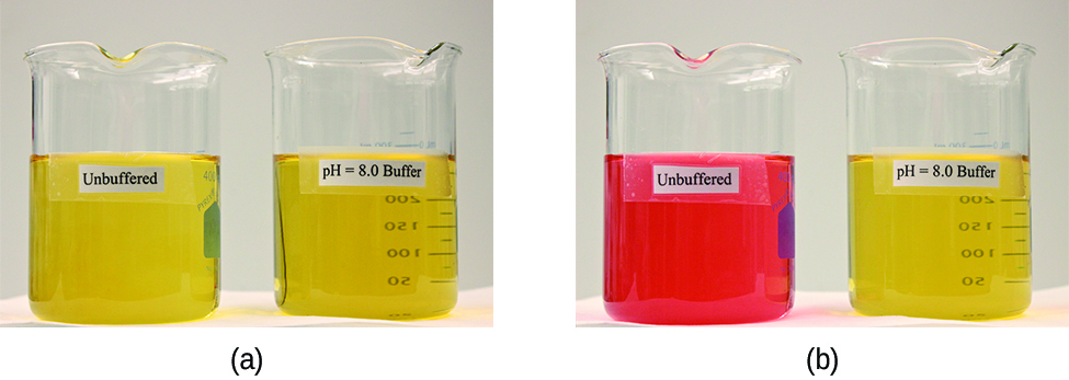
Two images are shown. Image a on the left shows two beakers that each contain yellow solutions. The beaker on the left is labeled “Unbuffered” and the beaker on the right is labeled “p H equals 8.0 buffer.” Image b similarly shows 2 beakers. The beaker on the left contains a bright orange solution and is labeled “Unbuffered.” The beaker on the right is labeled “p H equals 8.0 buffer.”
Figure 14.14 — 14.6

Figure 14.14 (a) The unbuffered solution on the left and the buffered solution on the right have the same pH (pH 8); they are basic, showing the yellow color of the indicator methyl orange at this pH. (b) After the addition of 1 mL of a 0.01- M HCl solution, the buffered solution has not detectably changed its pH but the unbuffered solution has become acidic, as indicated by the change in color of the methyl orange, which turns red at a pH of about 4. (credit: modification of work by Mark Ott)

Paul Flowers, Klaus Theopold, Richard Langley, and William R. Robinson, Chemistry 2E, OpenStax. (credit: modification of work by Mark Ott) · CC BY-NC-SA 4.0 · Original image ↗ · Access for free ↗
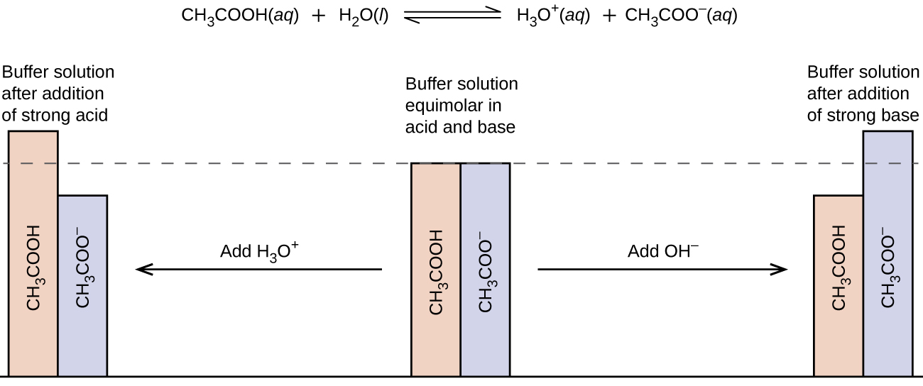
This figure begins with a chemical reaction at the top: C H subscript 3 C O O H ( a q ) plus H subscript 2 O ( l ) equilibrium arrow H subscript 3 O superscript positive sign ( a q ) plus C H subscript 3 C O O superscript negative sign ( a q ). Below the text is a figure that resembles a bar graph. In the middle are two bars of equal height. One is labeled, “C H subscript 3 C O O H,” and the other is labeled, “C H subscript 3 C O O superscript negative sign.” There is a dotted line at the same height of the bars which extends to the left and right. Above these two bars is the phrase, “Buffer solution equimolar in acid and base.” There is an arrow pointing to the right which is labeled, “Add O H superscript negative sign.” The arrow points to two bars again, but this time the C H subscript 3 C O O H bar is shorter than that C H subscript 3 C O O superscript negative sign bar. Above these two bars is the phrase, “Buffer solution after addition of strong base.” From the middle bars again, there is an arrow that points left. The arrow is labeled, “Add H subscript 3 O superscript positive sign.” This arrow points to two bars again, but this time the C H subscript 3 C O O H bar is taller than the C H subscript 3 C O O superscript negative sign bar. These two bars are labeled, “Buffer solution after addition of strong acid.”
Figure 14.15 — 14.6

Figure 14.15 Buffering action in a mixture of acetic acid and acetate salt.

Paul Flowers, Klaus Theopold, Richard Langley, and William R. Robinson, Chemistry 2E, OpenStax. · CC BY-NC-SA 4.0 · Original image ↗ · Access for free ↗
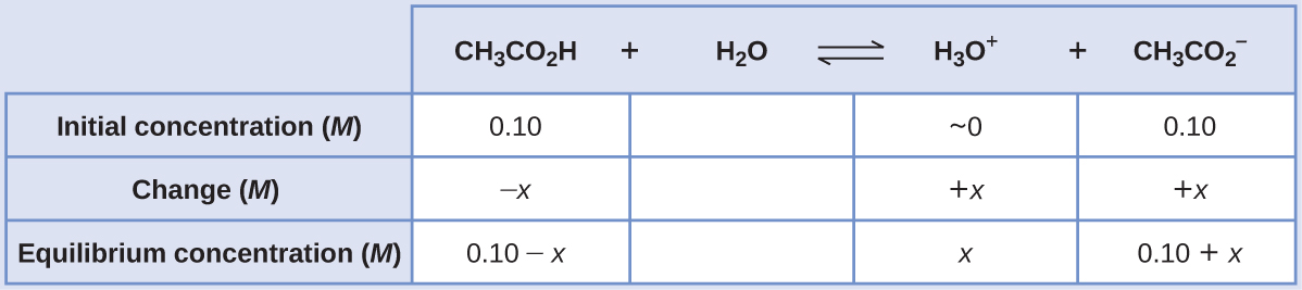
This table has two main columns and four rows. The first row for the first column does not have a heading and then has the following in the first column: Initial concentration ( M ), Change ( M ), Equilibrium concentration ( M ). The second column has the header of “[ C H subscript 3 C O subscript 2 H ] [ H subscript 2 O ] equilibrium arrow H subscript 3 O superscript plus sign [ C H subscript 3 C O subscript 2 superscript negative sign ].” Under the second column is a subgroup of four columns and three rows. The first column has the following: 0.10, negative x, 0.10 minus sign x. The second column is blank. The third column has the following: approximately 0, positive x, x. The fourth column has the following: 0.10, positive x, 0.10 plus sign x.
14.6 — illustration 3 Paul Flowers, Klaus Theopold, Richard Langley, and William R. Robinson, Chemistry 2E, OpenStax. · CC BY-NC-SA 4.0 · Original image ↗ · Access for free ↗
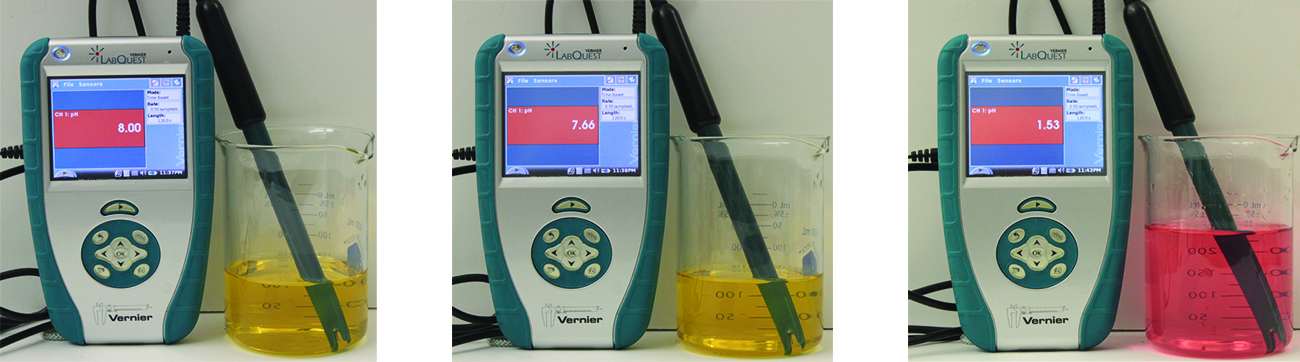
Three Vernier LabQuest devices measure pH: 8.00 (yellow solution), 7.66 (yellow solution), and 1.53 (red solution), demonstrating a range of pH values.
Figure 14.16 — 14.6

Figure 14.16 The indicator color (methyl orange) shows that a small amount of acid added to a buffered solution of pH 8 (beaker on the left) has little affect on the buffered system (middle beaker). However, a large amount of acid exhausts the buffering capacity of the solution and the pH changes dramatically (beaker on the right). (credit: modification of work by Mark Ott)

Paul Flowers, Klaus Theopold, Richard Langley, and William R. Robinson, Chemistry 2E, OpenStax. (credit: modification of work by Mark Ott) · CC BY-NC-SA 4.0 · Original image ↗ · Access for free ↗
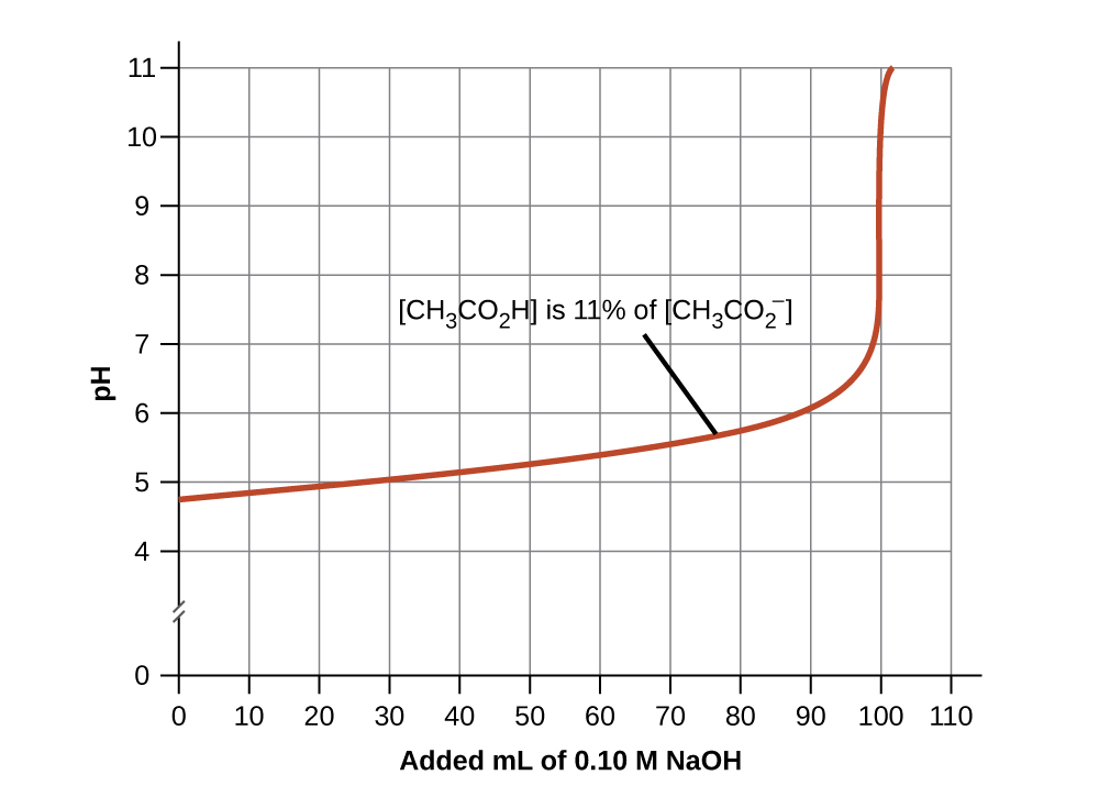
A graph is shown with a horizontal axis labeled “Added m L of 0.10 M N a O H” which has markings and vertical gridlines every 10 units from 0 to 110. The vertical axis is labeled “p H” and is marked every 1 unit beginning at 0 extending to 11. A break is shown in the vertical axis between 0 and 4. A red curve is drawn on the graph which increases gradually from the point (0, 4.8) up to about (100, 7) after which the graph has a vertical section up to about (100, 11). The curve is labeled [ C H subscript 3 C O subscript 2 H ] is 11 percent of [ C H subscript 3 CO subscript 2 superscript negative].
Figure 14.17 — 14.6

Figure 14.17 Change in pH as an increasing amount of a 0.10- M NaOH solution is added to 100 mL of a buffer solution in which, initially, [CH 3 CO 2 H] = 0.10 M and [ CH 3 CO 2 − ] = 0.10 M . [ CH 3 CO 2 − ] = 0.10 M . Note the greatly diminished buffering action occurring after the buffer capacity has been reached, resulting in drastic rises in pH on adding more strong base.

Paul Flowers, Klaus Theopold, Richard Langley, and William R. Robinson, Chemistry 2E, OpenStax. · CC BY-NC-SA 4.0 · Original image ↗ · Access for free ↗
Source: 14.6 Buffers

14.7 - Titrations — figures and tables

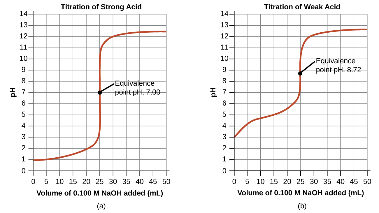
Two graphs are shown. The first graph on the left is titled “Titration of Weak Acid.” The horizontal axis is labeled “Volume of 0.100 M N a O H added (m L).” Markings and vertical gridlines are provided every 5 units from 0 to 50. The vertical axis is labeled “p H” and is marked every 1 unis beginning at 0 extending to 14. A red curve is drawn on the graph which increases steadily from the point (0, 3) up to about (20, 5.5) after which the graph has a vertical section from (25, 7) up to (25, 11). The graph then levels off to a value of about 12.5 from about 40 m L up to 50 m L. The midpoint of the vertical segment of the curve is labeled “Equivalence point p H, 8.72.” The second graph on the right is titled “Titration of Strong Acid.” The horizontal axis is labeled “Volume of 0.100 M N a O H added (m L).” Markings and vertical gridlines are provided every 5 units from 0 to 50. The vertical axis is labeled “p H” and is marked every 1 units beginning at 0 extending to 14. A red curve is drawn on the graph which increases gradually from the point (0, 1) up to about (22.5, 2.2) after which the graph has a vertical section from (25, 4) up to nearly (25, 11). The graph then levels off to a value of about 12.4 from about 40 m L up to 50 m L. The midpoint of the vertical segment of the curve is labeled “Equivalence point p H, 7.00.”
Figure 14.18 — 14.7 - Titrations

Figure 14.18 (a) The titration curve for the titration of 25.00 mL of 0.100 M HCl (strong acid) with 0.100 M NaOH (strong base) has an equivalence point of 7.00 pH. (b) The titration curve for the titration of 25.00 mL of 0.100 M acetic acid (weak acid) with 0.100 M NaOH (strong base) has an equivalence point of 8.72 pH.

Paul Flowers, Klaus Theopold, Richard Langley, and William R. Robinson, Chemistry 2E, OpenStax. · CC BY-NC-SA 4.0 · Original image ↗ · Access for free ↗
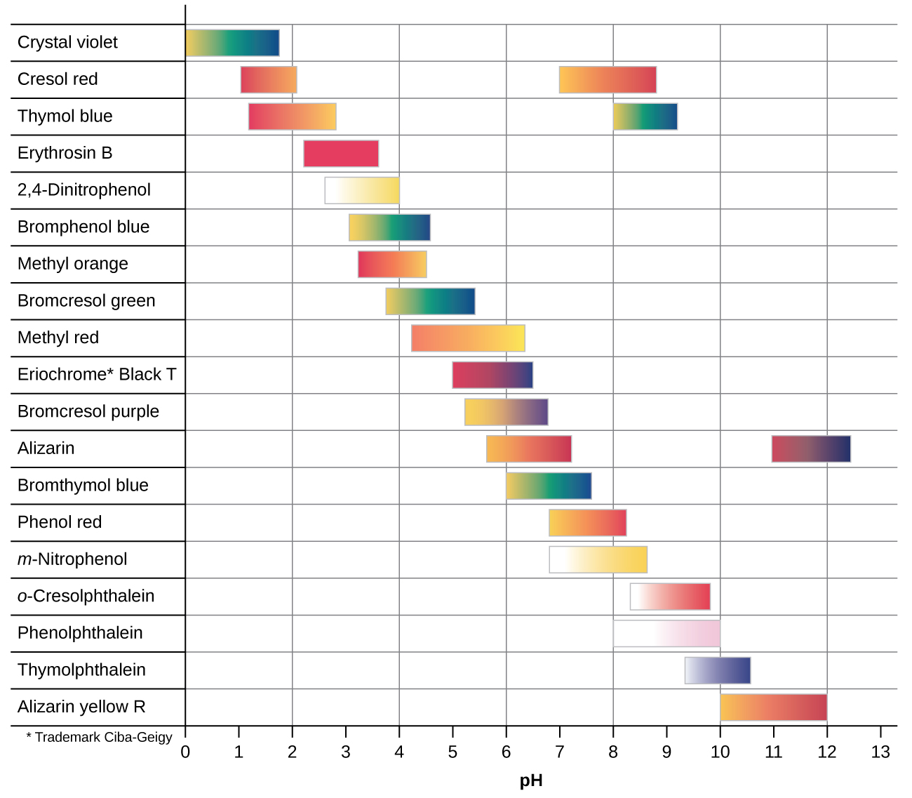
This figure provides a graphical representation of indicators and color ranges. A horizontal axis is labeled “p H.” This axis begins at zero and increases by ones up to 13. The left side of the graphic provides a column with the names of indicators. To the right of each indicator name is either one or two colored bars that are shaded according to the indicator color at various p H ranges. From the top, the first row is labeled “Crystal violet.” The associated colored bar is yellow at its left end at a p H of 0 and changes to green and blue moving right to its endpoint at a p H of 1.8. The second row is labeled “Cresol red.” The associated colored bar is red at its left end at a p H of 1 and changes to orange and yellow moving right to its endpoint at a p H of just over 2. A second bar to its right is yellow at a p H of around 7 and proceeds through orange to red at a p H of about 9. The third row is labeled “Thymol blue.” The associated colored bar is red at its left end at a p H of nearly 1.2 and changes to orange and red moving right to its endpoint at a p H of 2.8. A second bar begins in yellow at a p H of 8 and proceeds through green and blue to its end at a p H of around 9.1. The fourth row is labeled “Erythrosin B.” The associated colored bar is red from a p H of 2.2 to its endpoint at a p H of 3.6. The fifth row is labeled “2 comma 4 dash Dinitrophenol.” The associated colored bar is white at its left end at a p H of 2.6 and changes to yellow at its endpoint at a p H of 4. The sixth row is labeled “Bromophenol blue.” The associated colored bar is yellow at its left end at a p H of 3 and changes to green and blue moving right to its endpoint at a p H of 4.5. The seventh row is labeled “Methyl orange.” The associated colored bar is red-orange at its left end at a p H of 4.2 and changes to yellow moving right to its endpoint at a p H of 6.3. The eighth row is labeled “Bromocresol green.” The associated colored bar is yellow at its left end at a p H of 3.8 and changes to green and blue moving right to its endpoint at a p H of 5.4. The ninth row is labeled “Methyl red.” The associated colored bar is orange at its left end at a p H of 4.2 and changes to yellow moving right to its endpoint at a p H of 6.3. The tenth row is labeled “Eriochrome * Black T.” The associated colored bar is red at its left end at a p H of 5 and changes to purple and blue moving right to its endpoint at a p H of 6.5. The eleventh row is labeled “Bromocresol purple.” The associated colored bar is yellow at its left end at a p H of 5.2 and changes to purple moving right to its endpoint at a p H of 6.8. The twelfth row is labeled “Alizarin.” The first associated colored bar is yellow-orange at its left end at a p H of 5.7 and changes to red moving right to its endpoint at a p H of 7.2. A second bar begins in red at a p H of 11 and changes to purple, then dark blue at its right end at a p H of 12.4. The thirteenth row is labeled “Bromothymol blue.” The associated colored bar is yellow at its left end at a p H of 6 and changes to green and blue moving right to its endpoint at a p H of 7.6. The fourteenth row is labeled “Phenol red.” The associated colored bar is yellow-orange at its left end at a p H of 6.8 and changes to orange and red moving right to its endpoint at a p H of 8.2. The fifteenth row is labeled “m dash Nitrophenol.” The associated colored bar is white at its left end at a p H of 6.8 and changes to yellow moving right to its endpoint at a p H of 8.6. The sixteenth row is labeled “o dash Cresolphthalein.” The associated colored bar is white at its left end at a p H of 8.3 and changes to red moving right to its endpoint at a p H of 9.8. The seventeenth row is labeled “Phenolphthalein.” The associated colored bar is white at its left end at a p H of 8 and changes to pink moving right to its endpoint at a p H of 10. The eighteenth row is labeled “Thymolphthalein.” The associated colored bar is light blue at its left end at a p H of 9.3 and changes to a deep, dark blue moving right to its endpoint at a p H of 10.5. The nineteenth row is labeled “Alizarin yellow R.” The associated colored bar is yellow-orange at its left end at a p H of 10 and changes to red moving right to its endpoint at a p H of 12.
Figure 14.19 — 14.7 - Titrations

Figure 14.19 This chart illustrates the color change intervals for several acid-base indicators.

Paul Flowers, Klaus Theopold, Richard Langley, and William R. Robinson, Chemistry 2E, OpenStax. · CC BY-NC-SA 4.0 · Original image ↗ · Access for free ↗
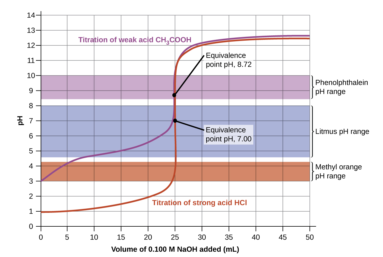
A graph is shown which is titled “Titration of Weak Acid.” The horizontal axis is labeled “Volume of 0.100 M N a O H added (m L)” and begins at 0 with markings every 5 units up to 50. The vertical axis is labeled “p H” and begins at 0 and increases by single units up to 14. A red curve is drawn on the graph. The curve begins at (0, 3) and passes through the points (5, 4.1), (10, 4.7), (15, 5), (20, 5.5), and (22.5, 6), after which it rapidly increases, forming a vertical section centered at the point (25, 8.7). The rapid increase of the curve then levels off and the curve passes through the points (30, 12), (35, 12.4), (40, 12.5), (45, 12.6), and (50, 12.6). A brown rectangle extends horizontally across the graph covering the p H of 3 to 4.2 range. To the right, this rectangle is labeled “Methyl orange p H range.” A blue rectangle extends horizontally across the graph covering the p H of 4.6 to 8 range. To the right, this rectangle is labeled “Litmus p H range.” A purple rectangle extends horizontally across the graph covering the p H of 8.4 to 10 range. To the right, this rectangle is labeled “Phenolphthalein p H range.” The midpoint of the vertical segment of the curve is labeled “Equivalence point p H, 8.72.”
Figure 14.20 — 14.7 - Titrations

Figure 14.20 Titration curves for strong and weak acids illustrating the proper choice of acid-base indicator. Any of the three indicators will exhibit a reasonably sharp color change at the equivalence point of the strong acid titration, but only phenolphthalein is suitable for use in the weak acid titration.

Paul Flowers, Klaus Theopold, Richard Langley, and William R. Robinson, Chemistry 2E, OpenStax. · CC BY-NC-SA 4.0 · Original image ↗ · Access for free ↗
Volume of 0.100 M NaOH Added (mL) Moles of NaOH Added Values 0.100 M HCl1 Values 0.100 M CH3CO2H2
0.0 0.0 1.00 2.87
5.0 0.00050 1.18 4.14
10.0 0.00100 1.37 4.57
15.0 0.00150 1.60 4.92
20.0 0.00200 1.95 5.35
22.0 0.00220 2.20 5.61
24.0 0.00240 2.69 6.13
24.5 0.00245 3.00 6.44
24.9 0.00249 3.70 7.14
25.0 0.00250 7.00 8.72
25.1 0.00251 10.30 10.30
25.5 0.00255 11.00 11.00
26.0 0.00260 11.29 11.29
28.0 0.00280 11.75 11.75
30.0 0.00300 11.96 11.96
35.0 0.00350 12.22 12.22
40.0 0.00400 12.36 12.36
45.0 0.00450 12.46 12.46
50.0 0.00500 12.52 12.52

Table 14.2. Paul Flowers, Klaus Theopold, Richard Langley, and William R. Robinson, Chemistry 2E, OpenStax.

Source: 14.7 Acid-Base Titrations

4.5 Chemical Analysis — figures and tables
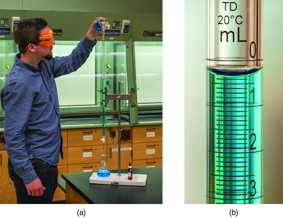
Two pictures are shown. In a, a person is shown pouring a liquid from a small beaker into a buret. The person is wearing goggles and gloves as she transfers the solution into the buret. In b, a close up view of the markings on the side of the buret is shown. The markings for 10, 15, and 20 are clearly shown with horizontal rings printed on the buret. Between each of these whole number markings, half markings are also clearly shown with horizontal line segment markings.
Figure 4.16 — 4.5 Chemical Analysis

Figure 4.16 (a) A student fills a buret in preparation for a titration analysis. (b) A typical buret permits volume measurements to the nearest 0.01 mL. (credit a: modification of work by Mark Blaser and Matt Evans; credit b: modification of work by Mark Blaser and Matt Evans)

Paul Flowers, Klaus Theopold, Richard Langley, and William R. Robinson, Chemistry 2E, OpenStax. (credit a: modification of work by Mark Blaser and Matt Evans; credit b: modification of work by Mark Blaser and Matt Evans) · CC BY-NC-SA 4.0 · Original image ↗ · Access for free ↗
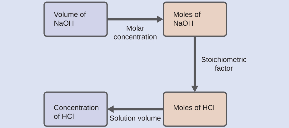
This figure shows four rectangles. The first is shaded lavender and is labeled, “Volume of N a O H.” This rectangle is followed by an arrow pointing right which is labeled, “Molar concentration,” to a second rectangle. This second rectangle is shaded pink and is labeled, “Moles of N a O H.” This rectangle is followed by an arrow pointing right which is labeled, “Stoichiometric factor,” to a third rectangle which is shaded pink and is labeled, “Moles of H C l.” This rectangle is followed by an arrow labeled, “Solution volume,” which points right to a fourth rectangle. This fourth rectangle is shaded lavender and is labeled, “Concentration of H C l.”
4.5 Chemical Analysis — illustration 2 Paul Flowers, Klaus Theopold, Richard Langley, and William R. Robinson, Chemistry 2E, OpenStax. · CC BY-NC-SA 4.0 · Original image ↗ · Access for free ↗
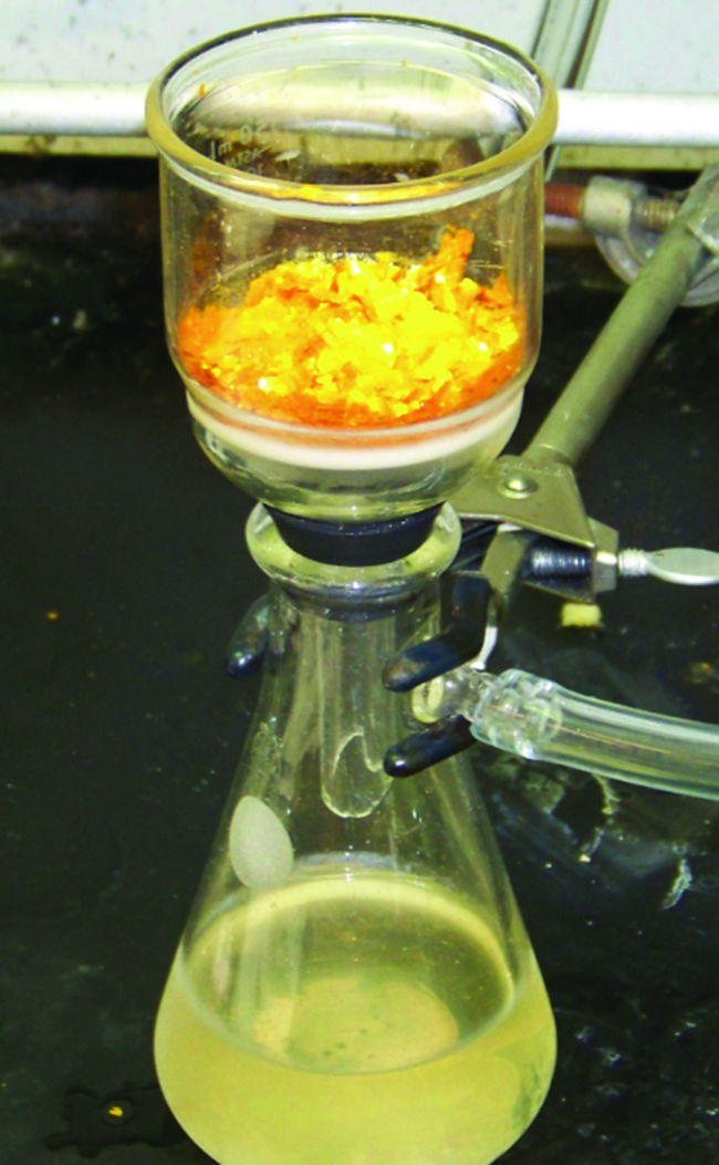
A photo is shown of a flask and funnel used for filtration. The flask contains a slightly opaque liquid filtrate with a slight yellow tint. A funnel, which contains a bright yellow and orange material, sits atop the flask. The flask is held in place by a clamp and is connected to a vacuum line. The connection between the funnel and flask is sealed with a rubber bung or gasket.
Figure 4.17 — 4.5 Chemical Analysis

Figure 4.17 Precipitate may be removed from a reaction mixture by filtration.

Paul Flowers, Klaus Theopold, Richard Langley, and William R. Robinson, Chemistry 2E, OpenStax. · CC BY-NC-SA 4.0 · Original image ↗ · Access for free ↗
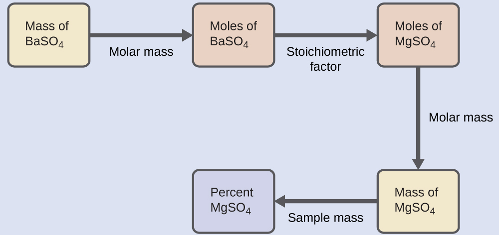
This figure shows five rectangles. The first is shaded yellow and is labeled “Mass of B a S O subscript 4.” This rectangle is followed by an arrow pointing right to a second rectangle. The arrow is labeled, “Molar mass.” The second rectangle is shaded pink and is labeled, “Moles of B a S O subscript 4.” This rectangle is followed by an arrow pointing right to a third rectangle. The arrow is labeled, “Stoichiometric factor.” This third rectangle is shaded pink and is labeled, “Moles of M g S O subscript 4.” This rectangle is followed by an arrow labeled, “Molar mass,” which points downward to a fourth rectangle. This fourth rectangle is shaded yellow and is labeled, “Mass of M g S O subscript 4.” This rectangle is followed by an arrow labeled, “Sample mass,” which points left to a fifth rectangle. This fifth rectangle is shaded lavender and is labeled, “Percent M g S O subscript 4.
4.5 Chemical Analysis — illustration 4 Paul Flowers, Klaus Theopold, Richard Langley, and William R. Robinson, Chemistry 2E, OpenStax. · CC BY-NC-SA 4.0 · Original image ↗ · Access for free ↗
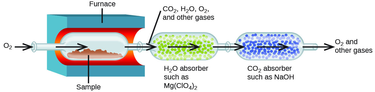
This diagram shows an arrow pointing from O subscript 2 into a tube that leads into a vessel containing a red material, labeled “Sample.” This vessel is inside a blue container with a red inner lining which is labeled “Furnace.” An arrow points from the tube to the right into the vessel above the red sample material. An arrow leads out of this vessel through a tube into a second vessel outside the furnace. An line points from this tube to a label above the diagram that reads “C O subscript 2, H subscript 2 O, O subscript 2, and other gases.” Many small green spheres are visible in the second vessel which is labeled below, “H subscript 2 O absorber such as M g ( C l O subscript 4 ) subscript 2.” An arrow points to the right through the vessel, and another arrow points right heading out of the vessel through a tube into a third vessel. The third vessel contains many small blue spheres. It is labeled “C O subscript 2 absorber such as N a O H.” An arrow points right through this vessel, and a final arrow points out of a tube at the right end of the vessel. Outside the end of this tube at the end of the arrow is the label, “O subscript 2 and other gases.”
Figure 4.18 — 4.5 Chemical Analysis

Figure 4.18 This schematic diagram illustrates the basic components of a combustion analysis device for determining the carbon and hydrogen content of a sample.

Paul Flowers, Klaus Theopold, Richard Langley, and William R. Robinson, Chemistry 2E, OpenStax. · CC BY-NC-SA 4.0 · Original image ↗ · Access for free ↗
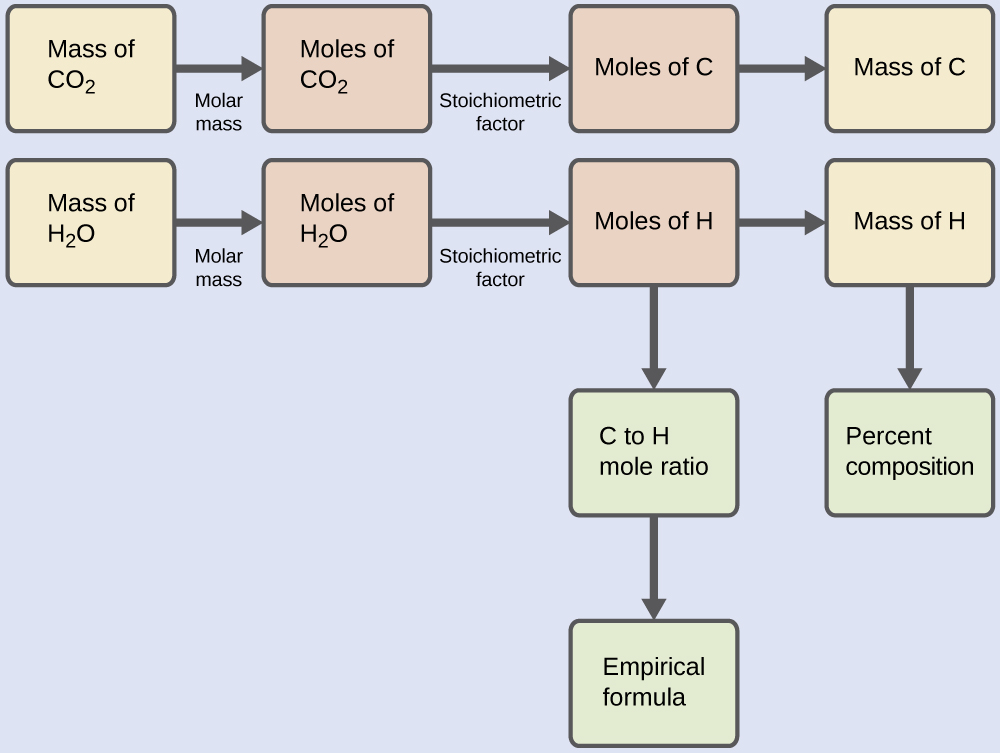
This figure shows two flowcharts. The first row is a single flow chart. In this row, a rectangle at the left is shaded yellow and is labeled, “Mass of C O subscript 2.” This rectangle is followed by an arrow pointing right to a second rectangle. The arrow is labeled, “Molar mass.” The second rectangle is shaded pink and is labeled, “Moles of C O subscript 2.” This rectangle is followed by an arrow pointing right to a third rectangle. The arrow is labeled, “Stoichiometric factor.” The third rectangle is shaded pink and is labeled, “Moles of C.” This rectangle is followed by an arrow labeled “Molar mass” which points right to a fourth rectangle. The fourth rectangle is shaded yellow and is labeled “Mass of C.” Below, is a second flowchart. It begins with a yellow shaded rectangle on the left which is labeled, “Mass of H subscript 2 O.” This rectangle is followed by an arrow labeled, “Molar mass,” which points right to a second rectangle. The second rectangle is shaded pink and is labeled, “Moles of H subscript 2 O.” This rectangle is followed by an arrow pointing right to a third rectangle. The arrow is labeled, “Stoichiometric factor.” The third rectangle is shaded pink and is labeled “Moles of H.” This rectangle is followed to the right by an arrow labeled, “Molar mass,” which points to a fourth rectangle. The fourth rectangle is shaded yellow and is labeled “Mass of H.” An arrow labeled, “Sample mass” points down beneath this rectangle to a green shaded rectangle. This rectangle is labeled, “Percent composition.” An arrow extends beneath the pink rectangle labeled, “Moles of H,” to a green shaded rectangle labeled, “C to H mole ratio.” Beneath this rectangle, an arrow extends to a second green shaded rectangle which is labeled, “Empirical formula.”
4.5 Chemical Analysis — illustration 6 Paul Flowers, Klaus Theopold, Richard Langley, and William R. Robinson, Chemistry 2E, OpenStax. · CC BY-NC-SA 4.0 · Original image ↗ · Access for free ↗

Source: 4.5 Quantitative Chemical Analysis

178 terms, alphabetically ordered

Acid · ·

In the Brønsted–Lowry model, a substance that can donate a . Acidic have a higher activity than water.

Read explanation · OpenStax ↗
acid dissociation constant

for an ’s -donation .

Read explanation · OpenStax ↗
Acid dissociation pKa · ·

The negative of an . At equal to pKa, an group is half .

Read explanation · OpenStax ↗
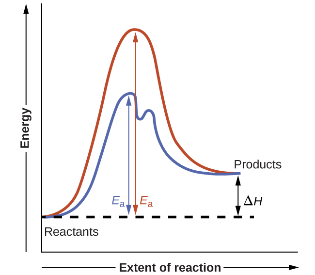
Activation energy ·

The energy barrier that must overcome to reach a and undergo .

Read explanation · OpenStax ↗
Active catalytic-site concentration ·

The total of active sites used to calculate from . It equals active when each has one site.

Read explanation · Biology LibreTexts ↗
Active site

The region of an that binds its and carries out .

Read explanation · OpenStax ↗
adaptation

A heritable feature shaped by selection because it improves reproductive success in a relevant environment.

Read explanation · OpenStax ↗
Adenosine triphosphate

An energy-carrying ; its powers many cellular processes, including cycles.

Read explanation · OpenStax ↗
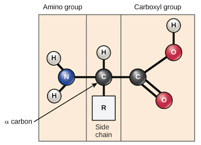
Alpha carbon · ·

The central carbon next to the carboxyl carbon. In a standard it binds an , hydrogen, and .

Read explanation · OpenStax ↗
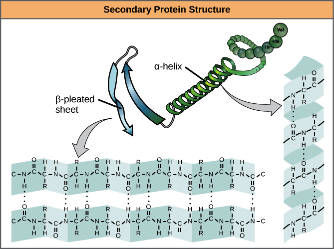
Alpha helix · · · · · ·

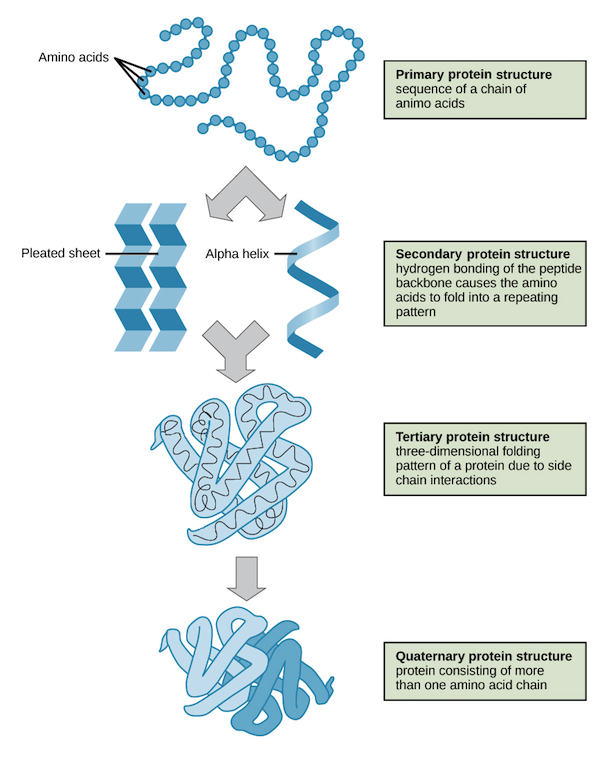
A helical stabilized by between a oxygen and an hydrogen four later.

Read explanation · OpenStax ↗
Amide · · ·

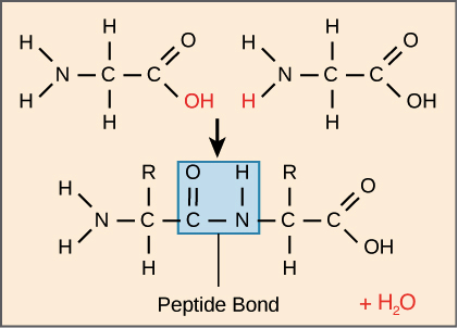
A group containing a carbon bonded to nitrogen. are amide linkages.

Read explanation · OpenStax ↗
Amino acid

A building block containing amino and and a characteristic .

Read explanation · OpenStax ↗
Amino acid residue · ·

The part of an incorporated into a chain. Residue can also describe another building block within a larger .

Read explanation · OpenStax ↗
Amino group · · ·

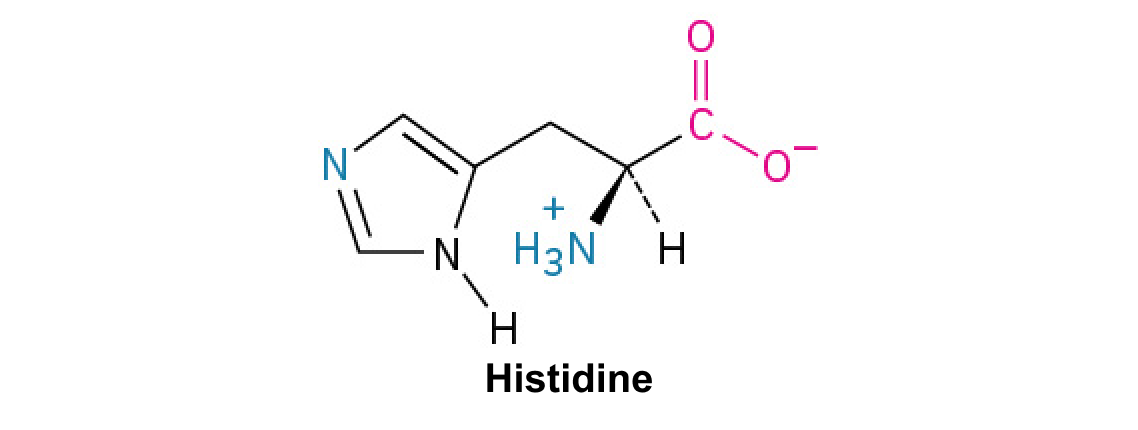
A nitrogen-containing . A free ’s amino group is typically (NH₃⁺) near physiological ; ’s ring nitrogen is an exception to this formula.

Read explanation · OpenStax ↗
Amphipathic

Having both a region and a region, as in a or .

Read explanation · OpenStax ↗
Analyte

A substance being measured or separated within a sample; the source table uses the term for the mixture under analysis.

Read explanation · Waters ↗
Analytical standard ·

A material with a known identity or amount used to compare or calibrate measurements.

Read explanation · Agilent ↗
Anion ·

An with a negative net .

Read explanation · OpenStax ↗
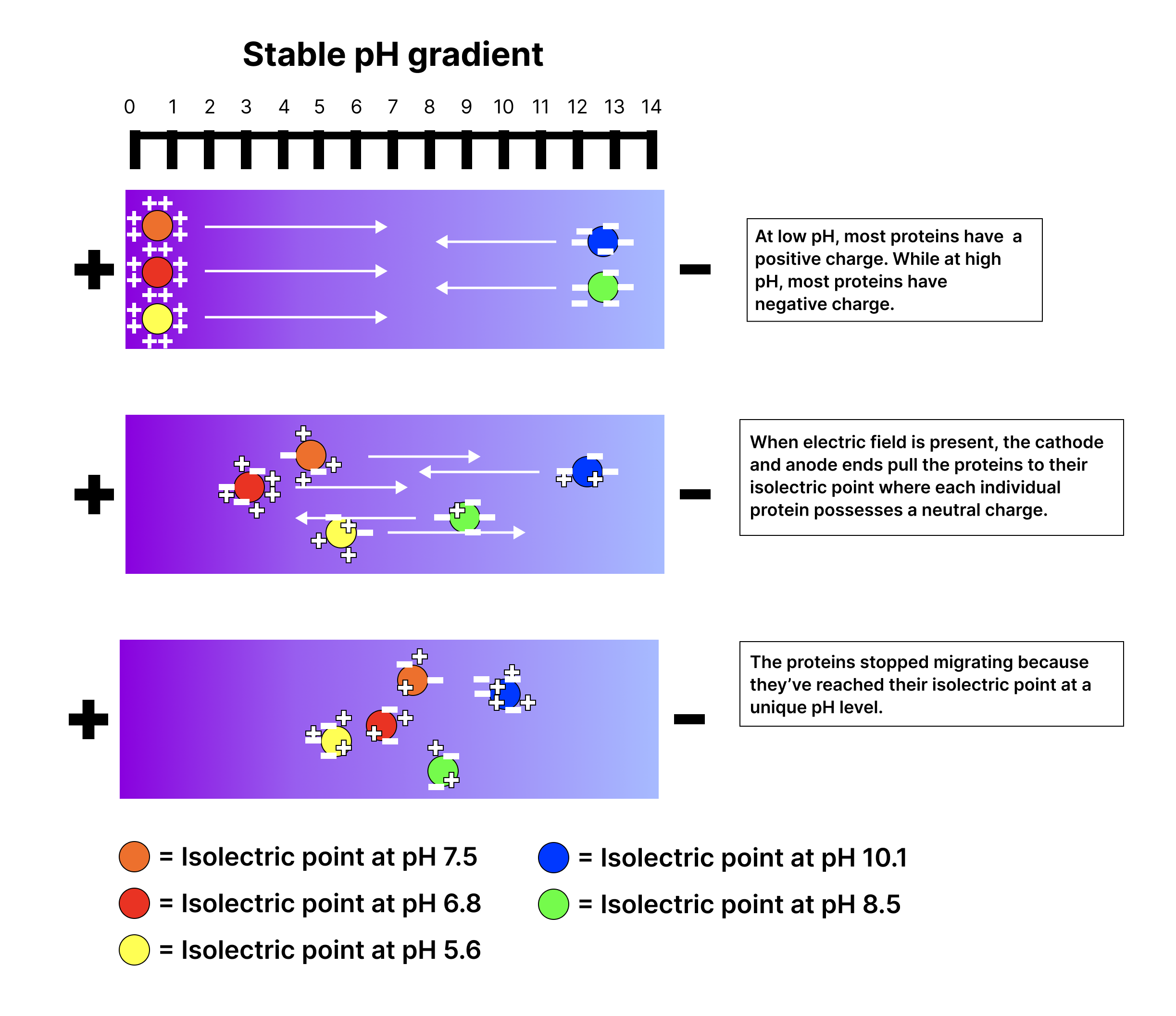
Anode

The positive in an apparatus; negatively migrate toward it.

Read explanation · Thermo Fisher ↗
Antiparallel

Running in opposite directions, as with two strands or neighboring strands in some .

Read explanation · OpenStax ↗
Aqueous solution ·

A in which water is the .

Read explanation · OpenStax ↗
Aromatic

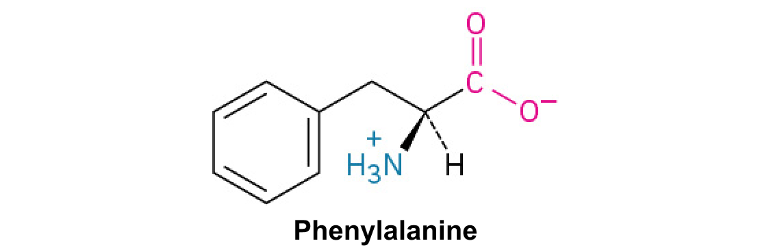
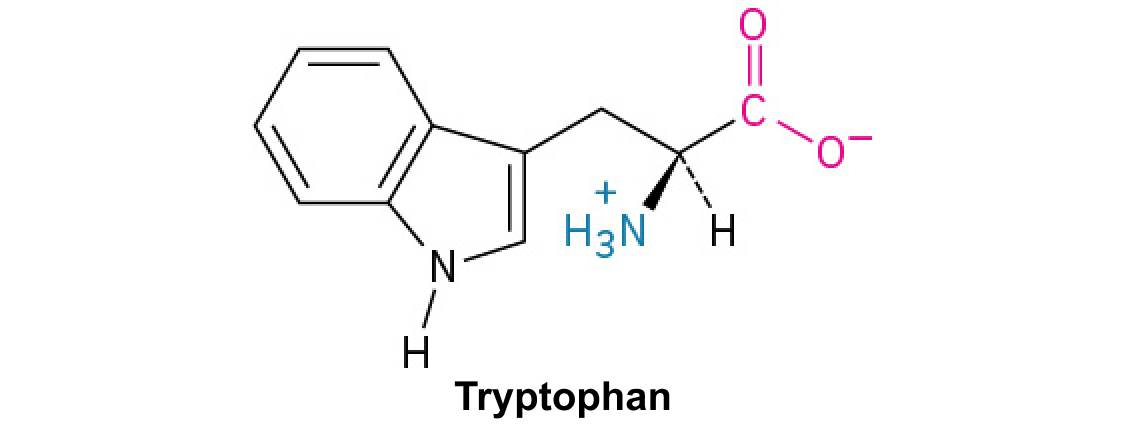
Containing a cyclic, with . , , and have aromatic .

Read explanation · OpenStax ↗
Atom

The smallest unit of an element that retains its chemical identity; it has a surrounded by .

Read explanation · OpenStax ↗
Benzene ring

A six-carbon ring with .

Read explanation · OpenStax ↗
Benzyl group

A attached through a –CH₂– group; part of ’s .

Read explanation · OpenStax ↗
Beta sheet · · · · · ·

A made of aligned segments connected by ; strands may be parallel or .

Read explanation · OpenStax ↗
bicarbonate ·

The HCO3− , a major extracellular component and form of carbon dioxide transport.

Read explanation · OpenStax ↗
Binding affinity ·

The strength of a binding interaction between . For simple binding, a smaller means higher affinity.

Read explanation · OpenStax ↗
Biomolecule

A made by or involved in living systems, including , , , and .

Read explanation · OpenStax ↗
Blotting ·

Transfer of separated or to a so a specific target can be detected.

Read explanation · Thermo Fisher ↗
Bohr effect

Reduced oxygen associated with increased CO2 or decreased .

Read explanation · OpenStax ↗
Brønsted–Lowry base · · · · · · · · · · ·

In the Brønsted–Lowry model, a substance that can accept a . Basic solutions have lower activity than water.

Read explanation · OpenStax ↗
Buffer ·

A that resists changes when small amounts of or are added, commonly through a weak and its .

Read explanation · OpenStax ↗
buffer capacity

Amount of added or a can absorb for a specified change.

Read explanation · OpenStax ↗
Calibration

Establishing the relation between a measured signal and known values or .

Read explanation · Agilent ↗
Carbohydrate

A class of including sugars and their , used for energy storage, structure, and recognition.

Read explanation · OpenStax ↗
Carbonyl group · ·

A carbon double-bonded to oxygen, C=O; present in and many other .

Read explanation · OpenStax ↗
Carboxyl group · ·

An , COOH. In free it is usually to COO⁻ near physiological .

Read explanation · OpenStax ↗
Catalyst · ·

A substance that speeds a by providing a pathway with lower and is regenerated rather than consumed overall.

Read explanation · OpenStax ↗
Cathode

The negative in an apparatus; positively migrate toward it.

Read explanation · Thermo Fisher ↗
Cation ·

An with a positive net .

Read explanation · OpenStax ↗
Chemical compound ·

A substance containing of two or more different chemically combined in a definite composition.

Read explanation · OpenStax ↗
Chemical element

A substance defined by having the same number of , such as carbon or oxygen.

Read explanation · OpenStax ↗
Chemical reaction ·

A process that rearranges and chemical bonds, converting into .

Read explanation · OpenStax ↗
Chromatin

The complex of and associated , including , in .

Read explanation · OpenStax ↗
Chromatography

Separation of mixture components by their different interactions with a and a moving .

Read explanation · Waters ↗
Chromatography resin ·

The solid or beads in a column, often carrying chemical groups that determine separation behavior.

Read explanation · Cytiva ↗
Chromosome ·

An organized with associated that carries . A replicated chromosome has two .

Read explanation · OpenStax ↗
Codon

A sequence of three that specifies an or a stop signal.

Read explanation · OpenStax ↗
Concentration

The amount of a substance in a specified volume or mass of mixture.

Read explanation · OpenStax ↗
conductor

Material with that can move readily through it.

Read explanation · OpenStax ↗
conjugate acid

Species formed when a gains one .

Read explanation · OpenStax ↗
conjugate base

Species formed when an loses one .

Read explanation · OpenStax ↗
Conjugated system ·

Adjacent orbitals that allow to be distributed across several , often through alternating single and multiple bonds.

Read explanation · OpenStax ↗
Covalent bond · ·

A bond in which share pairs. and are covalent.

Read explanation · OpenStax ↗
Cysteine ·

An with a . Two cysteines can form a .

Read explanation · OpenStax ↗
Deoxyribonucleic acid

The that stores genetic information used to specify and sequences.

Read explanation · OpenStax ↗
Deprotonation

Removal of a from a or group; this changes its by minus one.

Read explanation · OpenStax ↗
Detergent

An substance that can associate with both water and material; detergents can disrupt or interactions.

Read explanation · Thermo Fisher ↗
determination

Developmental commitment to a cell fate before all specialized features necessarily appear.

Read explanation · OpenStax ↗
Dissociation · ·

Separation of a chemical species or molecular complex into smaller components; dissociation releases a .

Read explanation · OpenStax ↗
Dissociation constant · ·

An for complex . For E + S ⇌ , Kd = [E]/[]; a smaller value indicates tighter binding under the stated conditions.

Read explanation · IUBMB ↗
Disulfide bond · · ·

A covalent sulfur–sulfur bond formed by of two , which can stabilize structure.

Read explanation · NCBI Bookshelf ↗
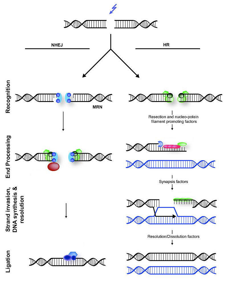
DNA replication

Copying so genetic information can be passed to daughter cells. Each guides a complementary new strand.

Read explanation · OpenStax ↗
Electric charge · · ·

An electrical property that can be positive or negative. Opposite charges attract and like charges repel; net charge is the sum of all charges on a particle.

Read explanation · OpenStax ↗
Electric field

A quantity describing the electrical force per unit positive . An applied field drives through a gel during .

Read explanation · Thermo Fisher ↗
Electrode

A that connects an electrical circuit to a or other medium; the and are electrodes.

Read explanation · Thermo Fisher ↗
Electron

A negatively subatomic particle. Electron sharing and transfer determine much of chemical bonding.

Read explanation · OpenStax ↗
Electron delocalization ·

Distribution of across several rather than confinement to one or bond.

Read explanation · OpenStax ↗
Electronegativity ·

An ’s tendency to attract shared in a chemical bond. Unequal attraction can make a bond .

Read explanation · OpenStax ↗
Electrophoresis

Movement of in an , used to separate through a support such as a gel.

Read explanation · Thermo Fisher ↗
empirical formula

Simplest whole-number atomic ratio in a .

Read explanation · OpenStax ↗
endpoint

Observed indicator or instrument change used to stop a .

Read explanation · OpenStax ↗
Enzyme

A biological that speeds a without being consumed. Most enzymes are .

Read explanation · OpenStax ↗
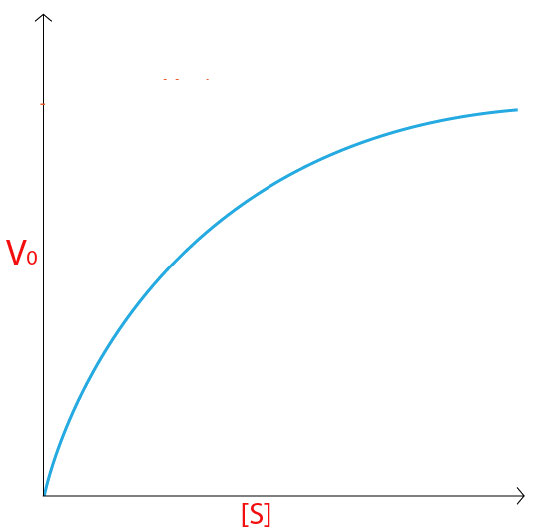
Enzyme saturation · ·

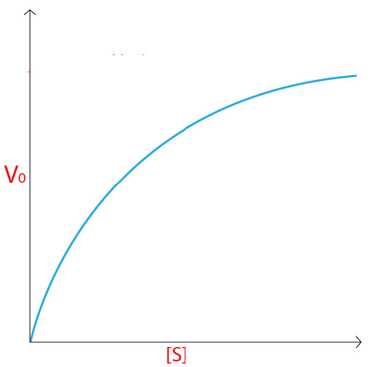
The high- limit in which sites spend almost all their time processing and the rate approaches .

Read explanation · Biology LibreTexts ↗
Enzyme–substrate complex · · ·

The bound association of an and its during a cycle. Often abbreviated ES in schemes.

Read explanation · OpenStax ↗
Equilibrium

A state where opposing processes occur at equal rates, so macroscopic or other properties remain constant.

Read explanation · OpenStax ↗
Equilibrium constant

A ratio of to activities at , each raised to its stoichiometric coefficient. At a fixed temperature, a does not change this ratio.

Read explanation · OpenStax ↗
equivalence point

point at which have combined in the stoichiometric ratio.

Read explanation · OpenStax ↗
Eukaryote ·

An organism whose cells have a -enclosed ; animals, plants, fungi, and protists are eukaryotes.

Read explanation · OpenStax ↗
Experimental control ·

A comparison sample or condition used to distinguish the effect being tested from other influences.

Read explanation · Thermo Fisher ↗
FACT complex ·

A -associated complex that helps machinery traverse and supports reorganization.

Read explanation · OpenStax ↗
Functional group

A group of whose chemical behavior gives a characteristic and properties.

Read explanation · OpenStax ↗
Gene

A sequence that contributes to a functional or , together with the information needed to express it.

Read explanation · OpenStax ↗
Gene expression

Production of a functional from a , including and, for -coding , .

Read explanation · NCBI Bookshelf ↗
half-equivalence point

Point halfway to equivalence in a simple weak- or weak- , where conjugate forms have equal amounts.

Read explanation · OpenStax ↗
Hemoglobin

The oxygen-carrying in , composed of four with heme groups.

Read explanation · OpenStax ↗
Henderson–Hasselbalch equation

Relationship = + log(activity of /activity of ), commonly approximated using .

Read explanation · OpenStax ↗
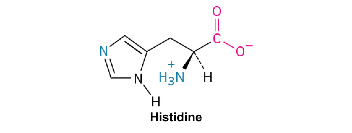
Histidine ·

A with an . Mostly uncharged near physiological , it can accept or donate .

Read explanation · OpenStax ↗
Histone

A -associated rich in . Core histones form the around which nucleosomal wraps.

Read explanation · OpenStax ↗
Hydrocarbon · ·

A made only of carbon and hydrogen. Hydrocarbon regions are generally .

Read explanation · OpenStax ↗
Hydrogen bond ·

An attraction between a hydrogen bonded to an and another . hydrogen bonds stabilize .

Read explanation · OpenStax ↗
Hydrogen ion · ·

A positively hydrogen species. H⁺ denotes a , which is hydrated in water; its activity determines .

Read explanation · OpenStax ↗
Hydrolysis

Breaking a chemical bond by adding water. hydrolysis separates .

Read explanation · OpenStax ↗
hydronium

H₃O⁺, a useful representation of a solvated in water.

Read explanation · OpenStax ↗
Hydrophilic

Interacting favorably with water, typically because a group is or .

Read explanation · OpenStax ↗
Hydrophobic

Interacting poorly with water. often gather in a ’s interior.

Read explanation · OpenStax ↗
Hydroxide ion ·

The negatively OH⁻. Basic contain a higher hydroxide ion activity than water at the same temperature.

Read explanation · OpenStax ↗
Hydroxyl group ·

An oxygen bonded to hydrogen, –OH. Hydroxyl groups can and often increase .

Read explanation · OpenStax ↗
Imidazole

A five-membered ring containing two nitrogens; ’s contains this ring.

Read explanation · OpenStax ↗
Indole

A fused six-membered and five-membered ring system containing nitrogen; found in .

Read explanation · OpenStax ↗
Ion · ·

An or with a net because its numbers of and do not balance.

Read explanation · OpenStax ↗
Ionization ·

Formation of electrically or , for example before analysis in a .

Read explanation · Thermo Fisher ↗
Le Châtelier’s principle

prediction that an composition shifts in response to a perturbation in a direction that reduces its effect.

Read explanation · OpenStax ↗
linkage

A tendency of nearby on the same to be inherited together.

Read explanation · OpenStax ↗
Lipid

A broad class of largely or , including fats, , and steroids.

Read explanation · OpenStax ↗
locus

The specific position of a or other feature.

Read explanation · OpenStax ↗
Logarithm · · ·

The exponent needed to obtain a number from a chosen fixed number. For decimal logarithms, log₁₀(100) = 2 because 10² = 100; uses the negative decimal logarithm of activity.

Read explanation · OpenStax ↗
Mass spectrometry ·

Analysis of according to their mass-to- ratios, used to identify and or .

Read explanation · Thermo Fisher ↗
Matrix

A supporting material, such as a gel or the solid support in a column. Its properties influence movement and binding of sample .

Read explanation · Thermo Fisher ↗
Maximum reaction rate · ·

The limiting as becomes saturating. For a fixed under given conditions, Vmax = times .

Read explanation · Biology LibreTexts ↗
Membrane · · · ·

A thin boundary or sheet. Cell membranes are bilayers containing ; membranes are synthetic supports that hold or for detection.

Read explanation · OpenStax ↗
Messenger RNA ·

An that carries coding information used by to synthesize a .

Read explanation · OpenStax ↗
Metabolism

The chemical that build , break them down, and transform energy in a living system.

Read explanation · OpenStax ↗
Methyl group ·

A –CH₃ group, consisting of one carbon bonded to three hydrogens.

Read explanation · OpenStax ↗
Mobile phase

The moving fluid that carries a sample through a system.

Read explanation · Waters ↗
molarity

Amount of in moles per liter of .

Read explanation · OpenStax ↗
mole

Amount containing exactly 6.02214076 × 10²³ specified entities.

Read explanation · OpenStax ↗
Molecular chaperone · ·

A that assists other in folding or prevents , without specifying their sequence.

Read explanation · NCBI Bookshelf ↗
Molecule

Two or more joined by . A molecule may be electrically or carry a .

Read explanation · OpenStax ↗
Neutral

Having no net . For a , neutral instead means equal and activities; its is about 7 at 25 °C.

Read explanation · OpenStax ↗
Nitrogenous base · · ·

A nitrogen-containing ring component of ; its pairing interactions help specify sequences.

Read explanation · OpenStax ↗
Nonpolar ·

Lacking a substantial separation of . Nonpolar groups generally interact poorly with water.

Read explanation · OpenStax ↗
Nucleic acid

A of , such as or , used in information storage, expression, and other cellular functions.

Read explanation · OpenStax ↗
Nucleosome

The basic unit of : wrapped around a .

Read explanation · OpenStax ↗
Nucleotide

A joined to a sugar and one or more .

Read explanation · OpenStax ↗
Nucleus ·

A -enclosed compartment containing most of a cell’s .

Read explanation · OpenStax ↗
Octamer

A complex made of eight . A core contains eight .

Read explanation · OpenStax ↗
Oxidation ·

Loss of or an increase in oxidation state. Oxidizing two can form a .

Read explanation · OpenStax ↗
Peptide

A chain of joined by ; the term commonly describes chains shorter than a typical .

Read explanation · OpenStax ↗
Peptide bond ·

A covalent between the carboxyl carbon of one and the amino nitrogen of the next.

Read explanation · OpenStax ↗
pH

A measure of , defined as the negative of activity. Lower pH means greater ; pH influences .

Read explanation · OpenStax ↗
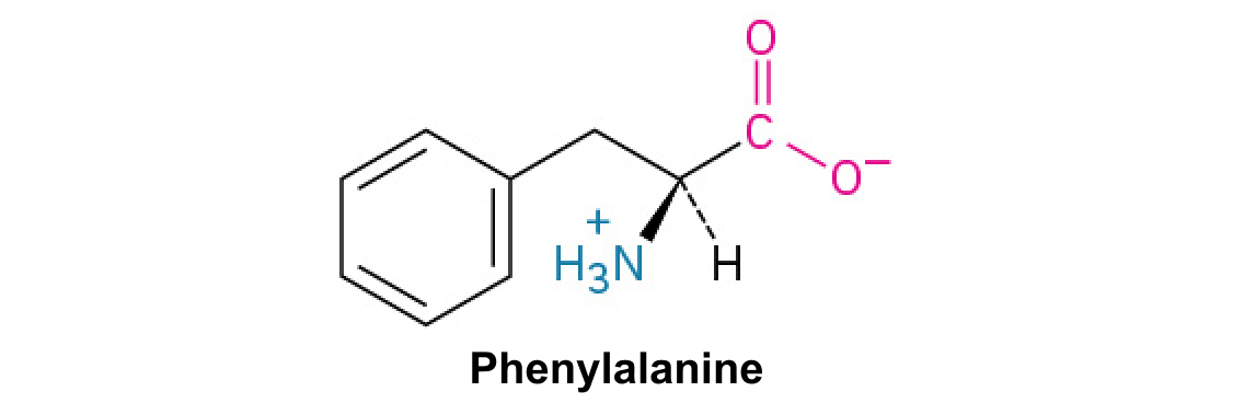
Phenylalanine ·

A with an .

Read explanation · OpenStax ↗
Phosphate group ·

A phosphorus-containing group bonded to oxygens; phosphate groups occur in , , and modified .

Read explanation · OpenStax ↗
Phospholipid

An with a -containing region and tails; a major component of cellular .

Read explanation · OpenStax ↗
Polar

Having an uneven distribution of . Polar groups often interact favorably with water.

Read explanation · OpenStax ↗
Polymer

A large made from many linked molecular building blocks.

Read explanation · OpenStax ↗
Polypeptide

A chain of connected by . A functional can contain one or several such chains.

Read explanation · OpenStax ↗
Porous material · · · ·

A material containing small spaces that can admit of suitable size.

Read explanation · Cytiva ↗
Proline ·

An whose loops back to the nitrogen, restricting rotation and often creating bends.

Read explanation · OpenStax ↗
Protein

One or more folded chains that perform biological roles such as , transport, signaling, or structural support.

Read explanation · OpenStax ↗
Protein aggregation · ·

Association of into larger clusters, often when exposed surfaces of unfolded stick together.

Read explanation · NCBI Bookshelf ↗
Protein backbone ·

The repeating nitrogen–alpha-carbon– chain of a , excluding its variable .

Read explanation · OpenStax ↗
Proton

A positively subatomic particle. In – chemistry, donating a proton means transferring a .

Read explanation · OpenStax ↗
Protonation

Addition of a to an , , or ; this changes its by plus one.

Read explanation · OpenStax ↗
Qualitative analysis

Analysis that identifies a substance or property without necessarily measuring its amount.

Read explanation · Agilent ↗
Quantification · ·

Estimating the amount or of a substance from measured signals and suitable or .

Read explanation · Waters ↗
R group · ·

The variable side chain attached to an ’s . It determines identity, , , and chemical behavior.

Read explanation · OpenStax ↗
Reactant

A starting substance transformed during a .

Read explanation · OpenStax ↗
Reaction intermediate · ·

A species formed in one step and consumed in another. It occupies a local energy minimum between .

Read explanation · OpenStax ↗
Reaction product ·

A substance formed by a .

Read explanation · OpenStax ↗
reaction quotient

-to- activity ratio with stoichiometric exponents at the current composition.

Read explanation · OpenStax ↗
Reaction rate · ·

How quickly are consumed or form, usually expressed as a change per unit time.

Read explanation · OpenStax ↗
Red blood cell · ·

A blood cell that transports oxygen using ; mature human red blood cells lack a .

Read explanation · OpenStax ↗
redox titration

based on a balanced -transfer .

Read explanation · OpenStax ↗
Reduction

Gain of or a decrease in state. Reducing a restores two .

Read explanation · OpenStax ↗
Ribonucleic acid ·

A with roles in , regulation, and ; carries -coding information.

Read explanation · OpenStax ↗
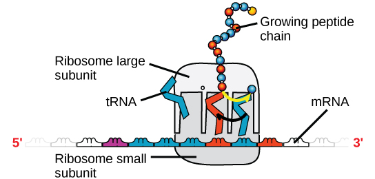
Ribosome ·

A complex of and that translates into a .

Read explanation · OpenStax ↗
Salt

An electrically made from and . Dissolved salts can screen or compete with – interactions.

Read explanation · Cytiva ↗
Secondary structure

Local folding, such as and , stabilized mainly by .

Read explanation · OpenStax ↗
Sister chromatid

One of the two copies of a produced by . An intact sister chromatid can supply a template for accurate repair.

Read explanation · Biology LibreTexts / Oregon State University ↗
Solubility ·

The amount of a substance that can dissolve in a under specified conditions. Soluble means able to dissolve; insoluble means only very slightly soluble in that .

Read explanation · OpenStax ↗
Solute

A dissolved component of a .

Read explanation · OpenStax ↗
Solution

A homogeneous mixture in which are dissolved in a .

Read explanation · OpenStax ↗
Solvent

The component of a that dissolves other substances, usually the component present in the greatest amount.

Read explanation · OpenStax ↗
Stationary phase

The material that remains fixed in a system.

Read explanation · Waters ↗
Substrate

A that an binds and chemically transforms.

Read explanation · OpenStax ↗
Substrate concentration

The amount of per volume. Square brackets denote ; [S] is varied to measure an curve.

Read explanation · Biology LibreTexts ↗
Subunit ·

An individual chain within a containing multiple chains.

Read explanation · OpenStax ↗
Template strand · · ·

A preexisting strand whose sequence guides complementary nucleic- synthesis.

Read explanation · OpenStax ↗
Thiol group · · · ·

A sulfur bonded to hydrogen, –SH. thiols can form through .

Read explanation · OpenStax ↗
Titration

Gradually adding a of known to another to measure its amount or – behavior.

Read explanation · OpenStax ↗
Transcription

Synthesis of using a template.

Read explanation · OpenStax ↗
Transition state

A fleeting, high-energy arrangement at a barrier. It is an energy maximum along the path, rather than a stable .

Read explanation · OpenStax ↗
Translation ·

Synthesis of a on a using the sequence of in .

Read explanation · OpenStax ↗
Tryptophan ·

An with a bulky ; commonly grouped as .

Read explanation · OpenStax ↗
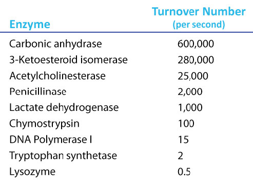
Turnover number · · ·

The maximum number of cycles per per unit time, calculated as /. Units are inverse time, commonly s⁻¹.

Read explanation · IUBMB ↗
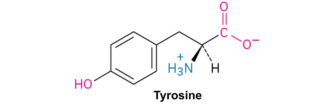
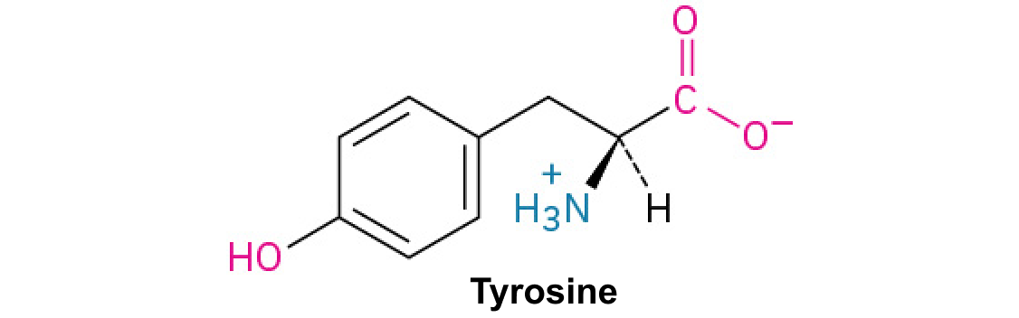
Tyrosine ·

An with a phenolic . Usually uncharged near physiological .

Read explanation · OpenStax ↗

14.6 Buffers

OpenStax · 14.6 Buffers ↗
Instructional page including learning objectives, examples, figures, source tables and questions. Site navigation and embedded media players are omitted; source media links remain available.

Learning Objectives

By the end of this section, you will be able to:

A containing appreciable amounts of a weak - pair is called a , or a . resist a change in when small amounts of a strong or a strong are added (Figure 14.14). A of acetic and sodium acetate (CH3 + CH3COONa) is an example of a that consists of a weak and its . An example of a that consists of a weak and its is a of ammonia and ammonium chloride (NH3(aq) + NH4Cl(aq)).

Two images are shown. Image a on the left shows two beakers that each contain yellow solutions. The beaker on the left is labeled “Unbuffered” and the beaker on the right is labeled “p H equals 8.0 buffer.” Image b similarly shows 2 beakers. The beaker on the left contains a bright orange solution and is labeled “Unbuffered.” The beaker on the right is labeled “p H equals 8.0 buffer.”
Figure 14.14 — 14.6

Figure 14.14 (a) The unbuffered solution on the left and the buffered solution on the right have the same pH (pH 8); they are basic, showing the yellow color of the indicator methyl orange at this pH. (b) After the addition of 1 mL of a 0.01- M HCl solution, the buffered solution has not detectably changed its pH but the unbuffered solution has become acidic, as indicated by the change in color of the methyl orange, which turns red at a pH of about 4. (credit: modification of work by Mark Ott)

Paul Flowers, Klaus Theopold, Richard Langley, and William R. Robinson, Chemistry 2E, OpenStax. (credit: modification of work by Mark Ott) · CC BY-NC-SA 4.0 · Original image ↗ · Access for free ↗

How Work

To illustrate the function of a , consider a mixture of roughly equal amounts of acetic and sodium acetate. The presence of a weak - pair in the imparts the ability to neutralize modest amounts of added strong or . For example, strong added to this will neutralize , causing the acetic to shift to the right and generate additional amounts of the weak (acetate ):

CH3CO2H(aq)+H2O(l)⇌H3O+(aq)+CH3CO2−(aq)

Likewise, strong added to this will shift the above left, producing additional amounts of the weak (acetic ). Figure 14.15 provides a graphical illustration of the changes in conjugate-partner that occur in this when strong and are added. The action of the is essentially a result of the added strong and being converted to the weak and that make up the 's conjugate pair. The weaker and undergo only slight , as compared with the complete of the strong and , and the , therefore, changes much less drastically than it would in an unbuffered .

This figure begins with a chemical reaction at the top: C H subscript 3 C O O H ( a q ) plus H subscript 2 O ( l ) equilibrium arrow H subscript 3 O superscript positive sign ( a q ) plus C H subscript 3 C O O superscript negative sign ( a q ). Below the text is a figure that resembles a bar graph. In the middle are two bars of equal height. One is labeled, “C H subscript 3 C O O H,” and the other is labeled, “C H subscript 3 C O O superscript negative sign.” There is a dotted line at the same height of the bars which extends to the left and right. Above these two bars is the phrase, “Buffer solution equimolar in acid and base.” There is an arrow pointing to the right which is labeled, “Add O H superscript negative sign.” The arrow points to two bars again, but this time the C H subscript 3 C O O H bar is shorter than that C H subscript 3 C O O superscript negative sign bar. Above these two bars is the phrase, “Buffer solution after addition of strong base.” From the middle bars again, there is an arrow that points left. The arrow is labeled, “Add H subscript 3 O superscript positive sign.” This arrow points to two bars again, but this time the C H subscript 3 C O O H bar is taller than the C H subscript 3 C O O superscript negative sign bar. These two bars are labeled, “Buffer solution after addition of strong acid.”
Figure 14.15 — 14.6

Figure 14.15 Buffering action in a mixture of acetic acid and acetate salt.

Paul Flowers, Klaus Theopold, Richard Langley, and William R. Robinson, Chemistry 2E, OpenStax. · CC BY-NC-SA 4.0 · Original image ↗ · Access for free ↗
Example 14.20

Changes in Buffered and Unbuffered

Acetate are used in biochemical studies of and other chemical components of cells to prevent changes that might affect the biochemical activity of these .

(a) Calculate the of an acetate that is a mixture with 0.10 M acetic and 0.10 M sodium acetate.

(b) Calculate the after 1.0 mL of 0.10 NaOH is added to 100 mL of this .

(c) For comparison, calculate the after 1.0 mL of 0.10 M NaOH is added to 100 mL of a of an unbuffered with a of 4.74.

(a) Following the ICE approach to this calculation yields the following:

Substituting the terms into the Ka expression, assuming x << 0.10, and solving the simplified equation for x yields

x=1.8×10⁻⁵M
[H3O+]=0+x=1.8×10⁻⁵M
pH=−log[H3O+]=−log(1.8×10⁻⁵)
=4.74

(b) Calculate the after 1.0 mL of 0.10 M NaOH is added to 100 mL of this .

Adding strong will neutralize some of the acetic , yielding the acetate . Compute the new of these two components, then repeat the calculation of part (a) using these new .

0.0010L×(0.10mol NaOH1L)=1.0×10⁻⁴mol NaOH

The initial molar amount of acetic is

0.100L×(0.100molCH3CO2H1L)=1.00×10⁻²molCH3CO2H

The amount of acetic remaining after some is neutralized by the added is

(1.0×10⁻²)−(0.01×10⁻²)=0.99×10⁻²molCH3CO2H

The newly formed acetate , along with the initially present acetate, gives a final acetate of

(1.0×10⁻²)+(0.01×10⁻²)=1.01×10⁻²molNaCH3CO2

Compute molar for the two components:

[CH3CO2H]=9.9×10⁻³mol0.101L=0.098M
[NaCH3CO2]=1.01×10⁻²mol0.101L=0.100M

Using these , the of the may be computed as in part (a) above, yielding = 4.75 (only slightly different from that prior to adding the strong ).

(c) For comparison, calculate the after 1.0 mL of 0.10 M NaOH is added to 100 mL of a of an unbuffered with a of 4.74.

The amount of initially present in the is

[ H 3 O + ]= 10 −4.74 =1.8× 10 −5 M
mol H 3 O + =(0.100L)(1.8× 10 −5 M)=1.8× 10 −6 mol H 3 O +

The amount of added to the is

mol OH − =(0.0010L)(0.10M)=1.0× 10 −4 mol OH −

The added hydroxide will neutralize via the

H 3 O + (aq)+ OH − (aq)⇋2 H 2 O(l)

The 1:1 stoichiometry of this shows that an excess of hydroxide has been added (greater molar amount than the initially present ).

The amount of remaining is

1.0× 10 −4 mol−1.8× 10 −6 mol=9.8× 10 −5 mol OH −

corresponding to a hydroxide of

9.8× 10 −5 mol OH − /0.101L=9.7× 10 −4 M

The of the is then calculated to be

pH=14.00−pOH=14.00−−log(9.7× 10 −4 )=10.99

In this unbuffered , addition of the results in a significant rise in (from 4.74 to 10.99) compared with the very slight increase observed for the in part (b) (from 4.74 to 4.75).

Check Your Learning

Show that adding 1.0 mL of 0.10 M HCl changes the of 100 mL of a 1.8 × 10⁻⁵ M HCl from 4.74 to 3.00.

Answer:

Initial of 1.8 × 10⁻⁵ M HCl; = −log[H3O+] = −log[1.8 × 10⁻⁵] = 4.74
Moles of H3O+ in 100 mL 1.8 × 10⁻⁵ M HCl; 1.8 × 10⁻⁵ moles/L × 0.100 L = 1.8 × 10⁻⁶
Moles of H3O+ added by addition of 1.0 mL of 0.10 M HCl: 0.10 moles/L × 0.0010 L = 1.0 × 10⁻⁴ moles; final after addition of 1.0 mL of 0.10 M HCl:

pH=−log[H3O+]=−log(total molesH3O+total volume)=−log(1.0×10⁻⁴mol+1.8×10⁻⁶mol101mL(1L1000mL))=3.00

do not have an unlimited capacity to keep the relatively constant (Figure 14.16). Instead, the ability of a to resist changes in relies on the presence of appreciable amounts of its conjugate weak - pair. When enough strong or is added to substantially lower the of either member of the pair, the action within the is compromised.

Three Vernier LabQuest devices measure pH: 8.00 (yellow solution), 7.66 (yellow solution), and 1.53 (red solution), demonstrating a range of pH values.
Figure 14.16 — 14.6

Figure 14.16 The indicator color (methyl orange) shows that a small amount of acid added to a buffered solution of pH 8 (beaker on the left) has little affect on the buffered system (middle beaker). However, a large amount of acid exhausts the buffering capacity of the solution and the pH changes dramatically (beaker on the right). (credit: modification of work by Mark Ott)

Paul Flowers, Klaus Theopold, Richard Langley, and William R. Robinson, Chemistry 2E, OpenStax. (credit: modification of work by Mark Ott) · CC BY-NC-SA 4.0 · Original image ↗ · Access for free ↗

The is the amount of or that can be added to a given volume of a before the changes significantly, usually by one unit. depends on the amounts of the weak and its that are in a mixture. For example, 1 L of a that is 1.0 M in acetic and 1.0 M in sodium acetate has a greater than 1 L of a that is 0.10 M in acetic and 0.10 M in sodium acetate even though both have the same . The first has more because it contains more acetic and acetate .

Selection of Suitable Mixtures

There are two useful rules of thumb for selecting mixtures:

  1. A good mixture should have about equal of both of its components. A has generally lost its usefulness when one component of the pair is less than about 10% of the other. Figure 14.17 shows how changes for an acetic -acetate as is added. The initial is 4.74. A change of 1 unit occurs when the acetic is reduced to 11% of the acetate .
    A graph is shown with a horizontal axis labeled “Added m L of 0.10 M N a O H” which has markings and vertical gridlines every 10 units from 0 to 110. The vertical axis is labeled “p H” and is marked every 1 unit beginning at 0 extending to 11. A break is shown in the vertical axis between 0 and 4. A red curve is drawn on the graph which increases gradually from the point (0, 4.8) up to about (100, 7) after which the graph has a vertical section up to about (100, 11). The curve is labeled [ C H subscript 3 C O subscript 2 H ] is 11 percent of [ C H subscript 3 CO subscript 2 superscript negative].
    Figure 14.17 — 14.6

    Figure 14.17 Change in pH as an increasing amount of a 0.10- M NaOH solution is added to 100 mL of a buffer solution in which, initially, [CH 3 CO 2 H] = 0.10 M and [ CH 3 CO 2 − ] = 0.10 M . [ CH 3 CO 2 − ] = 0.10 M . Note the greatly diminished buffering action occurring after the buffer capacity has been reached, resulting in drastic rises in pH on adding more strong base.

    Paul Flowers, Klaus Theopold, Richard Langley, and William R. Robinson, Chemistry 2E, OpenStax. · CC BY-NC-SA 4.0 · Original image ↗ · Access for free ↗
  2. Weak and their are better as for pHs less than 7; weak and their are better as for pHs greater than 7.

Blood is an important example of a buffered , with the principal and responsible for the action being carbonic , H2CO3, and the , HCO3−. When a is introduced to the blood stream, it is removed primarily by the :

H3O+(aq)+HCO3−(aq)⟶H2CO3(aq)+H2O(l)

An added is removed by the :

OH−(aq)+H2CO3(aq)⟶HCO3−(aq)+H2O(l)

The added strong or is thus effectively converted to the much weaker or of the pair (H3O+ is converted to H2CO3 and OH- is converted to HCO3-). The of human blood thus remains very near the value determined by the pairs , in this case, 7.35. Normal variations in blood are usually less than 0.1, and changes of 0.4 or greater are likely to be fatal.

The Henderson-Hasselbalch Equation

The -constant expression for a of a weak can be written as:

Ka=[H3O+][A−][HA]

Rearranging to solve for [H3O+] yields:

[H3O+]=Ka×[HA][A−]

Taking the negative of both sides of this equation gives

−log[H3O+]=−logKa− log[HA][A−],

which can be written as

pH=pKa+log[A−][HA]

where pKa is the negative of the of the constant of the weak (pKa = −log Ka). This equation relates the , the constant of a weak , and the of the weak - pair in a buffered . Scientists often use this expression, called the Henderson-Hasselbalch equation, to calculate the of . It is important to note that the “x is small” assumption must be valid to use this equation.

Portrait of a Chemist

Lawrence Joseph Henderson and Karl Albert Hasselbalch

Lawrence Joseph Henderson (1878–1942) was an American physician, biochemist and physiologist, to name only a few of many pursuits. He obtained a medical degree from Harvard and then spent 2 years studying in Strasbourg, then a part of Germany, before returning to take a lecturer position at Harvard. He eventually became a professor at Harvard and worked there entire life. He discovered that the - balance in human blood is regulated by a system formed by the dissolved carbon dioxide in blood. He wrote an equation in 1908 to describe the carbonic -carbonate system in blood. Henderson was broadly knowledgeable; in addition to important research on the physiology of blood, he also wrote on the of organisms and their fit with their environments, on sociology and on university education. He also founded the Fatigue Laboratory, at the Harvard Business School, which examined human physiology with specific focus on work in industry, exercise, and nutrition.

Karl Albert Hasselbalch (1874–1962), a Danish physician and chemist, shared authorship in a paper with Christian Bohr in 1904 that described the , which showed that the ability of in the blood to bind with oxygen was inversely related to the of the blood and the of carbon dioxide. The scale was introduced in 1909 by another Dane, Sørensen, and in 1912, Hasselbalch published measurements of the of blood. In 1916, Hasselbalch expressed Henderson’s equation in terms, consistent with the scale of , and thus the Henderson-Hasselbalch equation was born.

How Sciences Interconnect

Medicine: The System in Blood

The normal of human blood is about 7.4. The carbonate system in the blood uses the following :

CO2(g)+2H2O(l)⇌H2CO3(aq)⇌HCO3−(aq)+H3O+(aq)

The of carbonic , H2CO3 is approximately 0.0012 M, and the of the hydrogen carbonate , HCO3−, is around 0.024 M. Using the Henderson-Hasselbalch equation and the pKa of carbonic at body temperature, we can calculate the of blood:

pH=pKa+log[base][acid]=6.4+log0.0240.0012=7.7

The that the H2CO3 is significantly lower than that of the may seem unusual, but this imbalance is due to the that most of the by- of our that enter our bloodstream are . Therefore, there must be a larger proportion of than , so that the capacity of the will not be exceeded.

Lactic is produced in our muscles when we exercise. As the lactic enters the bloodstream, it is neutralized by the , producing H2CO3. An then accelerates the breakdown of the excess carbonic to carbon dioxide and water, which can be eliminated by breathing. In , in addition to the regulating effects of the carbonate system on the of blood, the body uses breathing to regulate blood . If the of the blood decreases too far, an increase in breathing removes CO2 from the blood through the lungs driving the such that [H3O+] is lowered. If the blood is too , a lower breath rate increases CO2 in the blood, driving the the other way, increasing [H+] and restoring an appropriate .

Link to Learning

View information on the system encountered in natural waters.

14.7 Acid-Base Titrations

OpenStax · 14.7 Acid-Base Titrations ↗
Instructional page including learning objectives, examples, figures, source tables and questions. Site navigation and embedded media players are omitted; source media links remain available.

Learning Objectives

By the end of this section, you will be able to:

As seen in the chapter on the stoichiometry of chemical , titrations can be used to quantitatively analyze for their or . In this section, we will explore the underlying chemical equilibria that make - titrimetry a useful analytical technique.

Curves

A is a plot of some property versus the amount of added titrant. For - titrations, is a useful property to monitor because it varies predictably with the composition and, therefore, may be used to monitor the ’s progress and detect its end point. The following example exercise demonstrates the computation of for a after additions of several specified titrant volumes. The first example involves a strong that requires only stoichiometric calculations to derive the . The second example addresses a weak requiring calculations.

Example 14.21

Calculating for : Strong /Strong

A is carried out for 25.00 mL of 0.100 M HCl (strong ) with 0.100 M of a strong NaOH (the is shown in Figure 14.18). Calculate the at these volumes of added :

(a) 0.00 mL

(b) 12.50 mL

(c) 25.00 mL

(d) 37.50 mL

(a) Titrant volume = 0 mL. The is due to the of HCl. Because this is a strong , the is complete and the is 0.100 M. The of the is then
pH=−log( 0.100 )=1.000

(b) Titrant volume = 12.50 mL. Since the sample and the titrant are both monoprotic and equally concentrated, this titrant addition involves less than a stoichiometric amount of , and so it is completely consumed by with the excess in the sample. The of remaining is computed by subtracting the consumed amount from the intial amount and then dividing by the volume:

[H3O+]=n(H+)V=0.002500 mol×(1000 mL1 L)−0.100M×12.50 mL25.00 mL+12.50 mL=0.0333M

(c) Titrant volume = 25.00 mL. This titrant addition involves a stoichiometric amount of (the ), and so only of the neutralization are in (water and NaCl). Neither the nor the of this undergo - ; the only process generating is the autoprotolysis of water. The is , having a = 7.00.

(d) Titrant volume = 37.50 mL. This involves the addition of titrant in excess of the . The is then calculated using the of :

n(OH−)0>n(H+)0
[OH−]=n(OH−)V=0.100M×37.50 mL−0.002500 mol×(1000 mL1 L)25.00 mL+37.50 mL=0.0200M

= 14 − pOH = 14 + log([OH−]) = 14 + log(0.0200) = 12.30

Check Your Learning

Calculate the for the strong /strong between 50.0 mL of 0.100 M HNO3(aq) and 0.200 M NaOH (titrant) at the listed volumes of added : 0.00 mL, 15.0 mL, 25.0 mL, and 40.0 mL.

Answer:

0.00: 1.000; 15.0: 1.5111; 25.0: 7; 40.0: 12.523

Example 14.22

of a Weak with a Strong

Consider the of 25.00 mL of 0.100 M CH3CO2H with 0.100 M NaOH. The can be represented as:
CH3CO2H+OH−⟶CH3CO2−+H2O

Calculate the of the after the addition of the following volumes of NaOH titrant:

(a) 0.00 mL

(b) 25.00 mL

(c) 12.50 mL

(d) 37.50 mL

(a) The initial is computed for the acetic in the usual ICE approach:

Ka=[H3O+][CH3CO2−][CH3CO2H]≈[H3O+]2[CH3CO2H]0, and [H3O+]=Ka×[CH3CO2H]=1.8×10−5×0.100=1.3×10⁻³

pH=−log(1.3×10⁻³)=2.87

(b) The and titrant are both monoprotic and the sample and titrant are equally concentrated; thus, this volume of titrant represents the . Unlike the strong- example above, however, the mixture in this case contains a weak (acetate ). The is computed considering the of acetate, which is present at a of

0.00250 mol0.0500 L=0.0500 MCH3CO2−

of acetate is represented by the equation

CH3CO2−(aq)+H2O(l)⇌CH3CO2H(aq)+OH−(aq)
Kb=[H+][OH−]Ka=KwKa=1.0×10−141.8×10−5=5.6×10⁻¹⁰

Assuming x << 0.0500, the may be calculated via the usual ICE approach: Kb=x20.0500M

x=[OH−]=5.3×10⁻⁶
pOH=−log(5.3×10⁻⁶)=5.28
pH=14.00−5.28=8.72

Note that the at the of this is significantly greater than 7, as expected when titrating a weak with a strong .

(c) Titrant volume = 12.50 mL. This volume represents one-half of the stoichiometric amount of titrant, and so one-half of the acetic has been neutralized to yield an equivalent amount of acetate . The of these - partners, therefore, are equal. A convenient approach to computing the is use of the Henderson-Hasselbalch equation:

pH=pKa+log[Base][Acid]=−log(Ka)+log[CH3CO2−][CH3CO2H]=−log(1.8×10⁻⁵)+log(1)
pH=−log(1.8×10⁻⁵)=4.74

( = pKa at the in a of a weak )

(d) Titrant volume = 37.50 mL. This volume represents a stoichiometric excess of titrant, and a containing both the , acetate , and the excess strong titrant. In such , the is determined primarily by the amount of excess strong :

[OH−]=(0.003750 mol−0.00250 mol)0.06250 L=2.00×10⁻²M
pOH=−log(2.00×10⁻²)=1.70, and pH=14.00−1.70=12.30

Check Your Learning

Calculate the for the weak /strong between 50.0 mL of 0.100 M HCOOH(aq) (formic ) and 0.200 M NaOH (titrant) at the listed volumes of added : 0.00 mL, 15.0 mL, 25.0 mL, and 30.0 mL.

Answer:

0.00 mL: 2.37; 15.0 mL: 3.92; 25.00 mL: 8.29; 30.0 mL: 12.097

Performing additional calculations similar to those in the preceding example permits a more full assessment of curves. A summary of /volume data pairs for the strong and weak titrations is provided in Table 14.2 and plotted as curves in Figure 14.18. A comparison of these two curves illustrates several important concepts that are best addressed by identifying the four stages of a :

initial state (added titrant volume = 0 mL): is determined by the being titrated; because the two samples are equally concentrated, the weak will exhibit a greater initial

pre- (0 mL < V < 25 mL): increases gradually and the is consumed by with added titrant; composition includes unreacted and the , its

(V = 25 mL): a drastic rise in is observed as the composition transitions from to either (for the strong sample) or basic (for the weak sample), with determined by of the of the

postequivalence point (V > 25 mL): is determined by the amount of excess strong titrant added; since both samples are titrated with the same titrant, both curves appear similar at this stage.

Values in the Titrations of a Strong and of a Weak
Volume of 0.100 M NaOH Added (mL) Moles of NaOH Added Values 0.100 M HCl1 Values 0.100 M CH3CO2H2
0.0 0.0 1.00 2.87
5.0 0.00050 1.18 4.14
10.0 0.00100 1.37 4.57
15.0 0.00150 1.60 4.92
20.0 0.00200 1.95 5.35
22.0 0.00220 2.20 5.61
24.0 0.00240 2.69 6.13
24.5 0.00245 3.00 6.44
24.9 0.00249 3.70 7.14
25.0 0.00250 7.00 8.72
25.1 0.00251 10.30 10.30
25.5 0.00255 11.00 11.00
26.0 0.00260 11.29 11.29
28.0 0.00280 11.75 11.75
30.0 0.00300 11.96 11.96
35.0 0.00350 12.22 12.22
40.0 0.00400 12.36 12.36
45.0 0.00450 12.46 12.46
50.0 0.00500 12.52 12.52
Table 14.2
Two graphs are shown. The first graph on the left is titled “Titration of Weak Acid.” The horizontal axis is labeled “Volume of 0.100 M N a O H added (m L).” Markings and vertical gridlines are provided every 5 units from 0 to 50. The vertical axis is labeled “p H” and is marked every 1 unis beginning at 0 extending to 14. A red curve is drawn on the graph which increases steadily from the point (0, 3) up to about (20, 5.5) after which the graph has a vertical section from (25, 7) up to (25, 11). The graph then levels off to a value of about 12.5 from about 40 m L up to 50 m L. The midpoint of the vertical segment of the curve is labeled “Equivalence point p H, 8.72.” The second graph on the right is titled “Titration of Strong Acid.” The horizontal axis is labeled “Volume of 0.100 M N a O H added (m L).” Markings and vertical gridlines are provided every 5 units from 0 to 50. The vertical axis is labeled “p H” and is marked every 1 units beginning at 0 extending to 14. A red curve is drawn on the graph which increases gradually from the point (0, 1) up to about (22.5, 2.2) after which the graph has a vertical section from (25, 4) up to nearly (25, 11). The graph then levels off to a value of about 12.4 from about 40 m L up to 50 m L. The midpoint of the vertical segment of the curve is labeled “Equivalence point p H, 7.00.”
Figure 14.18 — 14.7 - Titrations

Figure 14.18 (a) The titration curve for the titration of 25.00 mL of 0.100 M HCl (strong acid) with 0.100 M NaOH (strong base) has an equivalence point of 7.00 pH. (b) The titration curve for the titration of 25.00 mL of 0.100 M acetic acid (weak acid) with 0.100 M NaOH (strong base) has an equivalence point of 8.72 pH.

Paul Flowers, Klaus Theopold, Richard Langley, and William R. Robinson, Chemistry 2E, OpenStax. · CC BY-NC-SA 4.0 · Original image ↗ · Access for free ↗
- Indicators

Certain organic substances change color in dilute when the reaches a particular value. For example, phenolphthalein is a colorless substance in any with a greater than 5.0 × 10⁻⁹ M ( < 8.3). In more where the is less than 5.0 × 10⁻⁹ M ( > 8.3), it is red or pink. Substances such as phenolphthalein, which can be used to determine the of a , are called - indicators. - indicators are either weak organic or weak organic .

The in a of the - indicator orange, a weak , can be represented by an equation in which we use HIn as a simple representation for the complex orange :

HIn(aq)+H2O(l)⇌H3O+(aq)+In−(aq)redyellow
Ka=[H3O+][In−][HIn]=4.0×10⁻⁴

The of orange, In−, is yellow, and the nonionized form, HIn, is red. When we add to a of orange, the increased shifts the toward the nonionized red form, in accordance with . If we add , we shift the towards the yellow form. This behavior is completely analogous to the action of .

The perceived color of an indicator is determined by the ratio of the of the two species In− and HIn. If most of the indicator (typically about 60−90% or more) is present as In−, the perceived color of the is yellow. If most is present as HIn, then the color appears red. The Henderson-Hasselbalch equation is useful for understanding the relationship between the of an indicator and its composition (thus, perceived color):

pH=pKa+log([In−][HIn])

In where > pKa, the term must be positive, indicating an excess of the form of the indicator (yellow ). When < pKa, the log term must be negative, indicating an excess of the (red ). When the is close to the indicator , appreciable amounts of both conjugate partners are present, and the color is that of an additive combination of each (yellow and red, yielding orange). The color change interval (or interval) for an - indicator is defined as the range of values over which a change in color is observed, and for most indicators this range is approximately pKa ± 1.

There are many different - indicators that cover a wide range of values and can be used to determine the approximate of an unknown by a process of elimination. Universal indicators and paper contain a mixture of indicators and exhibit different colors at different pHs. Figure 14.19 presents several indicators, their colors, and their color-change intervals.

This figure provides a graphical representation of indicators and color ranges. A horizontal axis is labeled “p H.” This axis begins at zero and increases by ones up to 13. The left side of the graphic provides a column with the names of indicators. To the right of each indicator name is either one or two colored bars that are shaded according to the indicator color at various p H ranges. From the top, the first row is labeled “Crystal violet.” The associated colored bar is yellow at its left end at a p H of 0 and changes to green and blue moving right to its endpoint at a p H of 1.8. The second row is labeled “Cresol red.” The associated colored bar is red at its left end at a p H of 1 and changes to orange and yellow moving right to its endpoint at a p H of just over 2. A second bar to its right is yellow at a p H of around 7 and proceeds through orange to red at a p H of about 9. The third row is labeled “Thymol blue.” The associated colored bar is red at its left end at a p H of nearly 1.2 and changes to orange and red moving right to its endpoint at a p H of 2.8. A second bar begins in yellow at a p H of 8 and proceeds through green and blue to its end at a p H of around 9.1. The fourth row is labeled “Erythrosin B.” The associated colored bar is red from a p H of 2.2 to its endpoint at a p H of 3.6. The fifth row is labeled “2 comma 4 dash Dinitrophenol.” The associated colored bar is white at its left end at a p H of 2.6 and changes to yellow at its endpoint at a p H of 4. The sixth row is labeled “Bromophenol blue.” The associated colored bar is yellow at its left end at a p H of 3 and changes to green and blue moving right to its endpoint at a p H of 4.5. The seventh row is labeled “Methyl orange.” The associated colored bar is red-orange at its left end at a p H of 4.2 and changes to yellow moving right to its endpoint at a p H of 6.3. The eighth row is labeled “Bromocresol green.” The associated colored bar is yellow at its left end at a p H of 3.8 and changes to green and blue moving right to its endpoint at a p H of 5.4. The ninth row is labeled “Methyl red.” The associated colored bar is orange at its left end at a p H of 4.2 and changes to yellow moving right to its endpoint at a p H of 6.3. The tenth row is labeled “Eriochrome * Black T.” The associated colored bar is red at its left end at a p H of 5 and changes to purple and blue moving right to its endpoint at a p H of 6.5. The eleventh row is labeled “Bromocresol purple.” The associated colored bar is yellow at its left end at a p H of 5.2 and changes to purple moving right to its endpoint at a p H of 6.8. The twelfth row is labeled “Alizarin.” The first associated colored bar is yellow-orange at its left end at a p H of 5.7 and changes to red moving right to its endpoint at a p H of 7.2. A second bar begins in red at a p H of 11 and changes to purple, then dark blue at its right end at a p H of 12.4. The thirteenth row is labeled “Bromothymol blue.” The associated colored bar is yellow at its left end at a p H of 6 and changes to green and blue moving right to its endpoint at a p H of 7.6. The fourteenth row is labeled “Phenol red.” The associated colored bar is yellow-orange at its left end at a p H of 6.8 and changes to orange and red moving right to its endpoint at a p H of 8.2. The fifteenth row is labeled “m dash Nitrophenol.” The associated colored bar is white at its left end at a p H of 6.8 and changes to yellow moving right to its endpoint at a p H of 8.6. The sixteenth row is labeled “o dash Cresolphthalein.” The associated colored bar is white at its left end at a p H of 8.3 and changes to red moving right to its endpoint at a p H of 9.8. The seventeenth row is labeled “Phenolphthalein.” The associated colored bar is white at its left end at a p H of 8 and changes to pink moving right to its endpoint at a p H of 10. The eighteenth row is labeled “Thymolphthalein.” The associated colored bar is light blue at its left end at a p H of 9.3 and changes to a deep, dark blue moving right to its endpoint at a p H of 10.5. The nineteenth row is labeled “Alizarin yellow R.” The associated colored bar is yellow-orange at its left end at a p H of 10 and changes to red moving right to its endpoint at a p H of 12.
Figure 14.19 — 14.7 - Titrations

Figure 14.19 This chart illustrates the color change intervals for several acid-base indicators.

Paul Flowers, Klaus Theopold, Richard Langley, and William R. Robinson, Chemistry 2E, OpenStax. · CC BY-NC-SA 4.0 · Original image ↗ · Access for free ↗
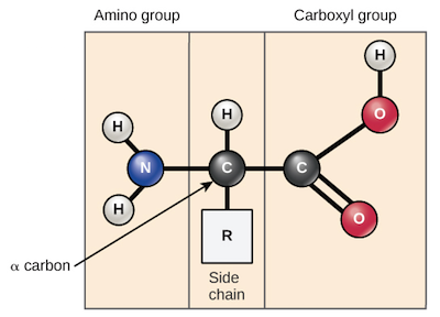
A graph is shown which is titled “Titration of Weak Acid.” The horizontal axis is labeled “Volume of 0.100 M N a O H added (m L)” and begins at 0 with markings every 5 units up to 50. The vertical axis is labeled “p H” and begins at 0 and increases by single units up to 14. A red curve is drawn on the graph. The curve begins at (0, 3) and passes through the points (5, 4.1), (10, 4.7), (15, 5), (20, 5.5), and (22.5, 6), after which it rapidly increases, forming a vertical section centered at the point (25, 8.7). The rapid increase of the curve then levels off and the curve passes through the points (30, 12), (35, 12.4), (40, 12.5), (45, 12.6), and (50, 12.6). A brown rectangle extends horizontally across the graph covering the p H of 3 to 4.2 range. To the right, this rectangle is labeled “Methyl orange p H range.” A blue rectangle extends horizontally across the graph covering the p H of 4.6 to 8 range. To the right, this rectangle is labeled “Litmus p H range.” A purple rectangle extends horizontally across the graph covering the p H of 8.4 to 10 range. To the right, this rectangle is labeled “Phenolphthalein p H range.” The midpoint of the vertical segment of the curve is labeled “Equivalence point p H, 8.72.”
Figure 14.20 — 14.7 - Titrations

Figure 14.20 Titration curves for strong and weak acids illustrating the proper choice of acid-base indicator. Any of the three indicators will exhibit a reasonably sharp color change at the equivalence point of the strong acid titration, but only phenolphthalein is suitable for use in the weak acid titration.

Paul Flowers, Klaus Theopold, Richard Langley, and William R. Robinson, Chemistry 2E, OpenStax. · CC BY-NC-SA 4.0 · Original image ↗ · Access for free ↗
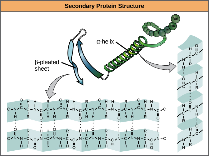
The curves shown in Figure 14.20 illustrate the choice of a suitable indicator for specific titrations. In the strong , use of any of the three indicators should yield reasonably sharp color changes and accurate end point determinations. For this , the reaches the lower limit of the orange color change interval after addition of ~24 mL of titrant, at which point the initially red would begin to appear orange. When 25 mL of titrant has been added (the ), the is well above the upper limit and the will appear yellow. The 's end point may then be estimated as the volume of titrant that yields a distinct orange-to-yellow color change. This color change would be challenging for most human eyes to precisely discern. More-accurate estimates of the end point are possible using either litmus or phenolphthalein, both of which exhibit color change intervals that are encompassed by the steep rise in that occurs around the 25.00 mL .

The weak in Figure 14.20 shows that only one of the three indicators is suitable for end point detection. If orange is used in this , the will undergo a gradual red-to-orange-to-yellow color change over a relatively large volume interval (0–6 mL), completing the color change well before the (25 mL) has been reached. Use of litmus would show a color change that begins after adding 7–8 mL of titrant and ends just before the . Phenolphthalein, on the other hand, exhibits a color change interval that nicely brackets the abrupt change in occurring at the 's . A sharp color change from colorless to pink will be observed within a very small volume interval around the .

4.5 Quantitative Chemical Analysis

OpenStax · 4.5 Quantitative Chemical Analysis ↗
Instructional page including learning objectives, examples, figures, source tables and questions. Site navigation and embedded media players are omitted; source media links remain available.

Learning Objectives

By the end of this section, you will be able to:

  • Describe the fundamental aspects of titrations and gravimetric analysis.
  • Perform stoichiometric calculations using typical and gravimetric data.

In the 18th century, the strength (actually the ) of vinegar samples was determined by noting the amount of potassium carbonate, K2CO3, which had to be added, a little at a time, before bubbling ceased. The greater the weight of potassium carbonate added to reach the point where the bubbling ended, the more concentrated the vinegar.

We now know that the effervescence that occurred during this process was due to with acetic , CH3CO2H, the primarily responsible for the odor and taste of vinegar. Acetic reacts with potassium carbonate according to the following equation:

2CH3CO2H(aq)+K2CO3(s)⟶2CH3CO2K(aq)+CO2(g)+H2O(l)

The bubbling was due to the production of CO2.

The test of vinegar with potassium carbonate is one type of analysis—the of the amount or of a substance in a sample. In the analysis of vinegar, the of the (acetic ) was determined from the amount of that combined with the present in a known volume of the . In other types of chemical analyses, the amount of a substance present in a sample is determined by measuring the amount of that results.

The described approach to measuring vinegar strength was an early version of the analytical technique known as analysis. A typical analysis involves the use of a buret (Figure 4.16) to make incremental additions of a containing a known of some substance (the titrant) to a sample containing the substance whose is to be measured (the ). The titrant and undergo a of known stoichiometry, and so measuring the volume of titrant required for complete with the (the of the ) allows calculation of the . The of a may be detected visually if a distinct change in the appearance of the sample accompanies the completion of the . The halt of bubble formation in the classic vinegar analysis is one such example, though, more commonly, special dyes called indicators are added to the sample to impart a change in color at or very near the of the . Equivalence points may also be detected by measuring some property that changes in a predictable way during the course of the . Regardless of the approach taken to detect a ’s , the volume of titrant actually measured is called the end point. Properly designed methods typically ensure that the difference between the equivalence and end points is negligible. Though any type of may serve as the basis for a analysis, the three described in this chapter (precipitation, -, and redox) are most common. Additional details regarding analysis are provided in the chapter on - equilibria.

Two pictures are shown. In a, a person is shown pouring a liquid from a small beaker into a buret. The person is wearing goggles and gloves as she transfers the solution into the buret. In b, a close up view of the markings on the side of the buret is shown. The markings for 10, 15, and 20 are clearly shown with horizontal rings printed on the buret. Between each of these whole number markings, half markings are also clearly shown with horizontal line segment markings.
Figure 4.16 — 4.5 Chemical Analysis

Figure 4.16 (a) A student fills a buret in preparation for a titration analysis. (b) A typical buret permits volume measurements to the nearest 0.01 mL. (credit a: modification of work by Mark Blaser and Matt Evans; credit b: modification of work by Mark Blaser and Matt Evans)

Paul Flowers, Klaus Theopold, Richard Langley, and William R. Robinson, Chemistry 2E, OpenStax. (credit a: modification of work by Mark Blaser and Matt Evans; credit b: modification of work by Mark Blaser and Matt Evans) · CC BY-NC-SA 4.0 · Original image ↗ · Access for free ↗

Example 4.14

Analysis

The end point in a of a 50.00-mL sample of aqueous HCl was reached by addition of 35.23 mL of 0.250 M NaOH titrant. The is:
HCl(aq)+NaOH(aq)⟶NaCl(aq)+H2O(l)

What is the of the HCl?

As for all stoichiometry calculations, the key issue is the relation between the molar amounts of the chemical species of interest as depicted in the balanced chemical equation. The approach outlined in previous modules of this chapter is followed, with additional considerations required, since the amounts of provided and requested are expressed as .

For this exercise, the calculation will follow the following outlined steps:

The molar amount of HCl is calculated to be:

35.23mL NaOH×1L1000mL×0.250mol NaOH1L×1 mol HCl1mol NaOH=8.81×10⁻³mol HCl

Using the provided volume of HCl and the definition of , the HCl is:

M=mol HClL solutionM=8.81×10⁻³mol HCl50.00 mL×1 L1000 mLM=0.176M

Note: For these types of calculations, it is convenient to recognize that is also equal to the number of millimoles of per milliliter of :

M=mol soluteL solution×103mmolmol103mLL=mmol solutemL solution

Using this version of the unit will shorten the calculation by eliminating two conversion factors:

35.23mL NaOH×0.250mmol NaOHmL NaOH×1mmol HCl1mmol NaOH50.00mL solution=0.176MHCl

Check Your Learning

A 20.00-mL sample of aqueous oxalic , H2C2O4, was titrated with a 0.09113-M of potassium permanganate, KMnO4 (see net ionic equation below).
2MnO4−(aq)+5H2C2O4(aq)+6H+(aq)⟶10CO2(g)+2Mn2+(aq)+8H2O(l)

A volume of 23.24 mL was required to reach the end point. What is the oxalic ?

Answer:

0.2648 M

Gravimetric Analysis

A gravimetric analysis is one in which a sample is subjected to some treatment that causes a change in the physical state of the that permits its separation from the other components of the sample. Mass measurements of the sample, the isolated , or some other component of the analysis system, used along with the known stoichiometry of the involved, permit calculation of the . Gravimetric methods were the first techniques used for chemical analysis, and they remain important tools in the modern chemistry laboratory.

The required change of state in a gravimetric analysis may be achieved by various physical and chemical processes. For example, the moisture (water) content of a sample is routinely determined by measuring the mass of a sample before and after it is subjected to a controlled heating process that evaporates the water. Also common are gravimetric techniques in which the is subjected to a precipitation of the sort described earlier in this chapter. The precipitate is typically isolated from the mixture by filtration, carefully dried, and then weighed (Figure 4.17). The mass of the precipitate may then be used, along with relevant stoichiometric relationships, to calculate .

A photo is shown of a flask and funnel used for filtration. The flask contains a slightly opaque liquid filtrate with a slight yellow tint. A funnel, which contains a bright yellow and orange material, sits atop the flask. The flask is held in place by a clamp and is connected to a vacuum line. The connection between the funnel and flask is sealed with a rubber bung or gasket.
Figure 4.17 — 4.5 Chemical Analysis

Figure 4.17 Precipitate may be removed from a reaction mixture by filtration.

Paul Flowers, Klaus Theopold, Richard Langley, and William R. Robinson, Chemistry 2E, OpenStax. · CC BY-NC-SA 4.0 · Original image ↗ · Access for free ↗
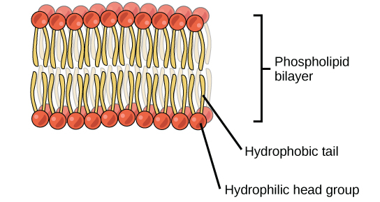
Example 4.15

Gravimetric Analysis

A 0.4550-g solid mixture containing MgSO4 is dissolved in water and treated with an excess of Ba(NO3)2, resulting in the precipitation of 0.6168 g of BaSO4.
MgSO4(aq)+Ba(NO3)2(aq)⟶BaSO4(s)+Mg(NO3)2(aq)

What is the (mass percent) of MgSO4 in the mixture?

The plan for this calculation is similar to others used in stoichiometric calculations, the central step being the connection between the moles of BaSO4 and MgSO4 through their stoichiometric factor. Once the mass of MgSO4 is computed, it may be used along with the mass of the sample mixture to calculate the requested percentage .

The mass of MgSO4 that would yield the provided precipitate mass is

0.6168g BaSO4×1mol BaSO4233.43g BaSO4×1mol MgSO41mol BaSO4×120.37g MgSO41mol MgSO4=0.3181g MgSO4

The of MgSO4 in the sample mixture is then calculated to be

percent MgSO4=mass MgSO4mass sample×100%0.3181 g0.4550 g×100%=69.91%

Check Your Learning

What is the percent of chloride in a sample if 1.1324 g of the sample produces 1.0881 g of AgCl when treated with excess Ag+?
Ag+(aq)+Cl−(aq)⟶AgCl(s)

Answer:

23.76%

The elemental composition of and related may be determined via a gravimetric method known as combustion analysis. In a combustion analysis, a weighed sample of the is heated to a high temperature under a stream of oxygen gas, resulting in its complete combustion to yield gaseous of known identities. The complete combustion of , for example, will yield carbon dioxide and water as the only . The gaseous combustion are swept through separate, preweighed collection devices containing that selectively absorb each (Figure 4.18). The mass increase of each device corresponds to the mass of the absorbed and may be used in an appropriate stoichiometric calculation to derive the mass of the relevant element.

This diagram shows an arrow pointing from O subscript 2 into a tube that leads into a vessel containing a red material, labeled “Sample.” This vessel is inside a blue container with a red inner lining which is labeled “Furnace.” An arrow points from the tube to the right into the vessel above the red sample material. An arrow leads out of this vessel through a tube into a second vessel outside the furnace. An line points from this tube to a label above the diagram that reads “C O subscript 2, H subscript 2 O, O subscript 2, and other gases.” Many small green spheres are visible in the second vessel which is labeled below, “H subscript 2 O absorber such as M g ( C l O subscript 4 ) subscript 2.” An arrow points to the right through the vessel, and another arrow points right heading out of the vessel through a tube into a third vessel. The third vessel contains many small blue spheres. It is labeled “C O subscript 2 absorber such as N a O H.” An arrow points right through this vessel, and a final arrow points out of a tube at the right end of the vessel. Outside the end of this tube at the end of the arrow is the label, “O subscript 2 and other gases.”
Figure 4.18 — 4.5 Chemical Analysis

Figure 4.18 This schematic diagram illustrates the basic components of a combustion analysis device for determining the carbon and hydrogen content of a sample.

Paul Flowers, Klaus Theopold, Richard Langley, and William R. Robinson, Chemistry 2E, OpenStax. · CC BY-NC-SA 4.0 · Original image ↗ · Access for free ↗

Example 4.16

Combustion Analysis

Polyethylene is a used to produce food-storage bags and many other flexible plastic items. A combustion analysis of a 0.00126-g sample of polyethylene yields 0.00394 g of CO2 and 0.00161 g of H2O. What is the of polyethylene?

The primary assumption in this exercise is that all the carbon in the sample combusted is converted to carbon dioxide, and all the hydrogen in the sample is converted to water:
CxHy(s)+excess O2(g)⟶xCO2(g)+y2H2O(g)

Note that a balanced equation is not necessary for the task at hand. To derive the of the , only the subscripts x and y are needed.

First, calculate the molar amounts of carbon and hydrogen in the sample, using the provided masses of the carbon dioxide and water, respectively. With these molar amounts, the for the may be written as described in the previous chapter of this text. An outline of this approach is given in the following flow chart:

mol C=0.00394g CO2×1mol CO244.01 g×1mol C1mol CO2=8.95×10⁻⁵mol Cmol H=0.00161g H2O×1mol H2O18.02g×2mol H1mol H2O=1.79×10⁻⁴mol H

The for the is then derived by identifying the smallest whole-number multiples for these molar amounts. The H-to-C molar ratio is

mol Hmol C=1.79×10⁻⁴mol H8.95×10−5mol C=2mol H1mol C

and the for polyethylene is CH2.

Check Your Learning

A 0.00215-g sample of polystyrene, a composed of carbon and hydrogen, produced 0.00726 g of CO2 and 0.00148 g of H2O in a combustion analysis. What is the for polystyrene?

Answer:

CH