Foundation 4 · 4B · Fluids, gases, and circulation

Molecular gas behavior

Sources ↗

Temperature fixes average translational ; mass changes the speed needed for that energy.

Microscopic motion and

For particles, average translational is 3kBT/2 per particle; = R/NA. is vrms = √(3RT/M), with M in kg/mol. Lighter move faster at the same temperature, but have the same average translational . A monatomic has U = 3nRT/2 and molar CV = 3R/2. At constant pressure the gas also expands, so CP = CV + R. Molecular rotations and vibrations add available energy modes; heat capacities can therefore depend on molecular structure and temperature.

Source: 9.5 The Kinetic-Molecular Theory · 9.6 Non-Ideal Gas Behavior · 13.4 Kinetic Theory: Atomic and Molecular Explanation of Pressure and Temperature

When ideal assumptions fail

Real gases depart most strongly from ideality at high pressure and low temperature. Intermolecular attractions reduce the pressure of a given sample relative to noninteracting particles; excluded molecular volume becomes important when particles crowd together. The van der Waals model is (P + an²/V²)(V − nb) = nRT. The parameter a corrects attraction and b corrects excluded volume; neither is universal. Compressibility Z = PV/(nRT) equals one for an and can fall below or rise above one for real gases.

Source: 9.5 The Kinetic-Molecular Theory · 9.6 Non-Ideal Gas Behavior · 13.4 Kinetic Theory: Atomic and Molecular Explanation of Pressure and Temperature

Apply it

Try before revealing the answer. At the same temperature, compare vrms of helium (4 g/mol) and oxygen (32 g/mol). How much does a monatomic ’s molar change when heated by 20 K?

Worked answer

vHe/vO₂ = √(32/4) = √8 ≈ 2.83. Equal temperature means equal average translational , not equal speed. ΔUmolar = (3/2)RΔT ≈ 1.5 × 8.314 × 20 = 249 J/mol.

Source: 9.5 The Kinetic-Molecular Theory · 9.6 Non-Ideal Gas Behavior · 13.4 Kinetic Theory: Atomic and Molecular Explanation of Pressure and Temperature

9.5 The -Molecular Theory — figures and tables

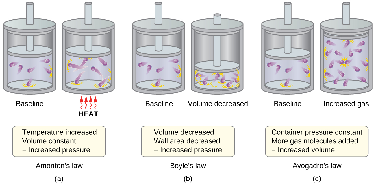
This figure shows 3 pairs of pistons and cylinders. In a, which is labeled, “Charles’s Law,” the piston is positioned for the first cylinder so that just over half of the available volume contains 6 purple spheres with trails behind them. The trails indicate movement. Orange dashes extend from the interior surface of the cylinder where the spheres have collided. This cylinder is labeled, “Baseline.” In the second cylinder, the piston is in the same position, and the label, “Heat” is indicated in red capitalized text. Four red arrows with wavy stems are pointing upward to the base of the cylinder. The six purple spheres have longer trails behind them and the number of orange dashes indicating points of collision with the container walls has increased. A rectangle beneath the diagram states, “Temperature increased, Volume constant equals Increased pressure.” In b, which is labeled, “Boyle’s Law,” the first, baseline cylinder shown is identical to the first cylinder in a. In the second cylinder, the piston has been moved, decreasing the volume available to the 6 purple spheres to half of the initial volume. The orange dashes indicating points of collision with the container walls has increased. This second cylinder is labeled, “Volume decreased.” A rectangle beneath the diagram states, “Volume decreased, Wall area decreased equals Increased pressure.” In c, which is labeled “Avogadro’s Law,” the first, baseline cylinder shown is identical to the first cylinder in a. In the second cylinder, the number of purple spheres has changed from 6 to 12 and volume has doubled. This second cylinder is labeled “Increased gas.” A rectangle beneath the diagram states, “At constant pressure, More gas molecules added equals Increased volume.”
Figure 9.31 — 9.5 The -Molecular Theory

Figure 9.31 (a) When gas temperature increases, gas pressure increases due to increased force and frequency of molecular collisions. (b) When volume decreases, gas pressure increases due to increased frequency of molecular collisions. (c) When the amount of gas increases at a constant pressure, volume increases to yield a constant number of collisions per unit wall area per unit time.

Paul Flowers, Klaus Theopold, Richard Langley, and William R. Robinson, Chemistry 2E, OpenStax. · CC BY-NC-SA 4.0 · Original image ↗ · Access for free ↗
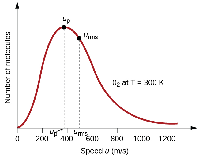
A graph is shown. The horizontal axis is labeled, “Speed u ( m divided by s ).” This axis is marked by increments of 20 beginning at 0 and extending up to 120. The vertical axis is labeled, “Fraction of molecules.” A positively or right-skewed curve is shown in red which begins at the origin and approaches the horizontal axis around 120 m per s. At the peak of the curve, a point is indicated with a black dot and is labeled, “v subscript p.” A vertical dashed line extends from this point to the horizontal axis at which point the intersection is labeled, “v subscript p.” Slightly to the right of the peak a second black dot is placed on the curve. This point is labeled, “v subscript r m s.” A vertical dashed line extends from this point to the horizontal axis at which point the intersection is labeled, “v subscript r m s.” The label, “O subscript 2 at T equals 300 K” appears in the open space to the right of the curve.
Figure 9.32 — 9.5 The -Molecular Theory

Figure 9.32 The molecular speed distribution for oxygen gas at 300 K is shown here. Very few molecules move at either very low or very high speeds. The number of molecules with intermediate speeds increases rapidly up to a maximum, which is the most probable speed, then drops off rapidly. Note that the most probable speed, ν p , is a little less than 400 m/s, while the root mean square speed, u rms , is closer to 500 m/s.

Paul Flowers, Klaus Theopold, Richard Langley, and William R. Robinson, Chemistry 2E, OpenStax. · CC BY-NC-SA 4.0 · Original image ↗ · Access for free ↗
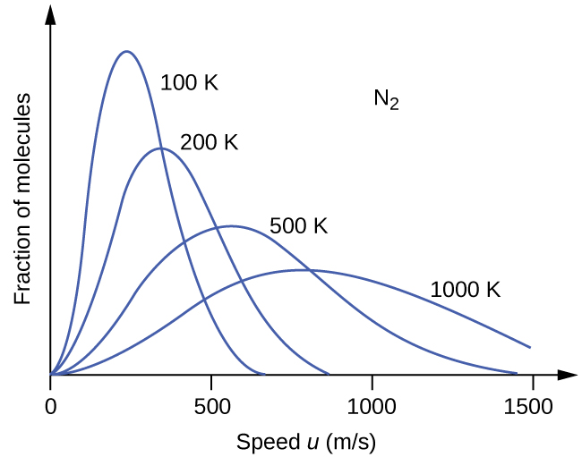
A graph with four positively or right-skewed curves of varying heights is shown. The horizontal axis is labeled, “Speed u ( m divided by s ).” This axis is marked by increments of 500 beginning at 0 and extending up to 1500. The vertical axis is labeled, “Fraction of molecules.” The label, “N subscript 2,” appears in the open space in the upper right area of the graph. The tallest and narrowest of these curves is labeled, “100 K.” Its right end appears to touch the horizontal axis around 700 m per s. It is followed by a slightly wider curve which is labeled, “200 K,” that is about three quarters of the height of the initial curve. Its right end appears to touch the horizontal axis around 850 m per s. The third curve is significantly wider and only about half the height of the initial curve. It is labeled, “500 K.” Its right end appears to touch the horizontal axis around 1450 m per s. The final curve is only about one third the height of the initial curve. It is much wider than the others, so much so that its right end has not yet reached the horizontal axis. This curve is labeled, “1000 K.”
Figure 9.33 — 9.5 The -Molecular Theory

Figure 9.33 The molecular speed distribution for nitrogen gas (N 2 ) shifts to the right and flattens as the temperature increases; it shifts to the left and heightens as the temperature decreases.

Paul Flowers, Klaus Theopold, Richard Langley, and William R. Robinson, Chemistry 2E, OpenStax. · CC BY-NC-SA 4.0 · Original image ↗ · Access for free ↗
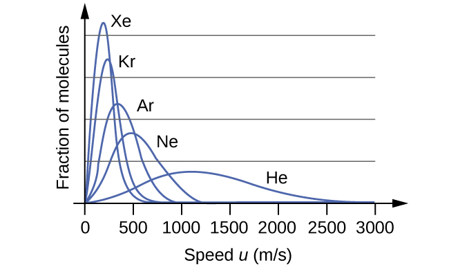
A graph is shown with four positively or right-skewed curves of varying heights. The horizontal axis is labeled, “Speed u ( m divided by s ).” This axis is marked by increments of 500 beginning at 0 and extending up to 3000. The vertical axis is labeled, “Fraction of molecules.” The tallest and narrowest of these curves is labeled, “X e.” Its right end appears to touch the horizontal axis around 600 m per s. It is followed by a slightly wider curve which is labeled, “A r,” that is about half the height of the initial curve. Its right end appears to touch the horizontal axis around 900 m per s. The third curve is significantly wider and just over a third of the height of the initial curve. It is labeled, “N e.” Its right end appears to touch the horizontal axis around 1200 m per s. The final curve is only about one fourth the height of the initial curve. It is much wider than the others, so much so that its right reaches the horizontal axis around 2500 m per s. This curve is labeled, “H e.”
Figure 9.34 — 9.5 The -Molecular Theory

Figure 9.34 molecular speed is directly related to molecular mass. At a given temperature, lighter molecules move faster on average than heavier molecules.

Paul Flowers, Klaus Theopold, Richard Langley, and William R. Robinson, Chemistry 2E, OpenStax. · CC BY-NC-SA 4.0 · Original image ↗ · Access for free ↗
Source: 9.5 The Kinetic-Molecular Theory

9.6 Non- Behavior — figures and tables

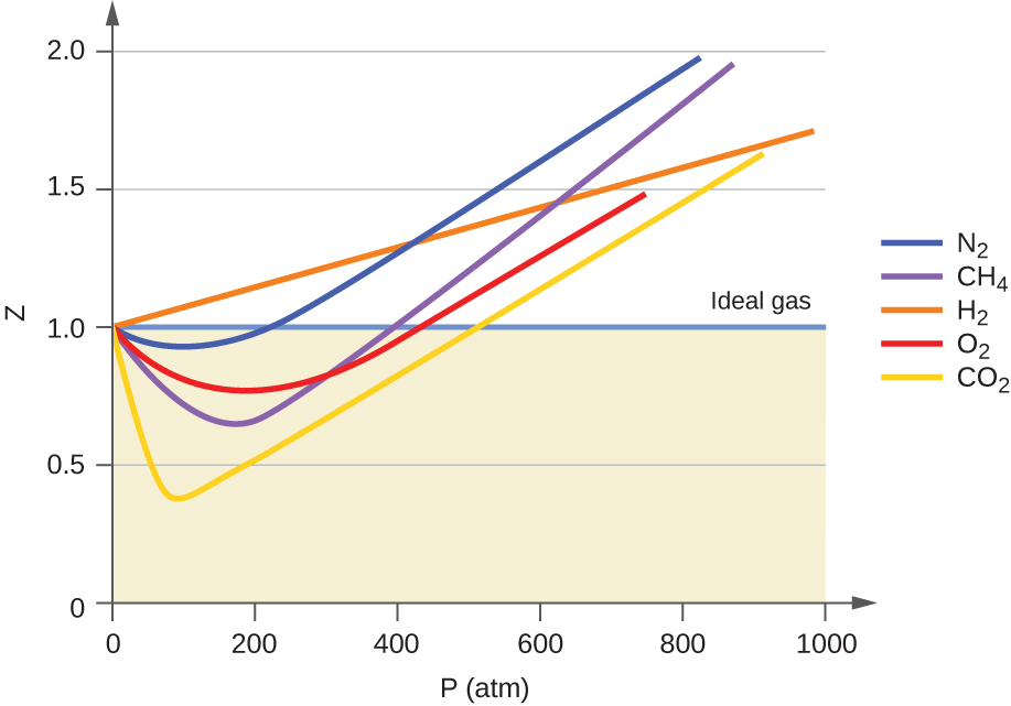
A graph is shown. The horizontal axis is labeled, “P ( a t m ).” Its scale begins at zero with markings provided by multiples of 200 up to 1000. The vertical axis is labeled, “Z le( k P a ).” This scale begins at zero and includes multiples of 0.5 up to 2.0. Six curves are drawn of varying colors. One of these curves is a horizontal, light purple line extending right from 1.0 k P a on the vertical axis, which is labeled “Ideal gas.” The region of the graph beneath this line is shaded tan. The remaining curves also start at the same point on the vertical axis. An orange line extends to the upper right corner of the graph, reaching a value of approximately 1.7 k P a at 1000 a t m. This orange curve is labeled, “H subscript 2.” A blue curve dips below the horizontal ideal gas line initially, then increases to cross the line just past 200 a t m. This curve reaches a value of nearly 2.0 k P a at about 800 a t m. This curve is labeled, “N subscript 2.” A red curve dips below the horizontal ideal gas line initially, then increases to cross the line just past 400 a t m. This curve reaches a value of nearly 1.5 k P a at about 750 a t m. This curve is labeled, “O subscript 2.” A purple curve dips below the horizontal ideal gas line, dipping even lower than the O subscript 2 curve initially, then increases to cross the ideal gas line at about 400 a t m. This curve reaches a value of nearly 2.0 k P a at about 850 a t m. This curve is labeled, “C H subscript 4.” A yellow curve dips below the horizontal ideal gas line, dipping lower than the other curves to a minimum of about 0.4 k P a at about 0.75 a t m, then increases to cross the ideal gas line at about 500 a t m. This curve reaches a value of about 1.6 k P a at about 900 a t m. This curve is labeled, “C O subscript 2.”
Figure 9.35 — 9.6 Non- Behavior

Figure 9.35 A graph of the compressibility factor (Z) vs. pressure shows that gases can exhibit significant deviations from the behavior predicted by the ideal gas law.

Paul Flowers, Klaus Theopold, Richard Langley, and William R. Robinson, Chemistry 2E, OpenStax. · CC BY-NC-SA 4.0 · Original image ↗ · Access for free ↗

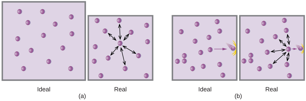
This figure includes two diagrams. Each involves two lavender shaded boxes that contain 14 relatively evenly distributed, purple spheres. The first box in a on the left is labeled “ideal.” In the second slightly smaller box, on the right, a nearly centrally located purple sphere has 6 double-headed arrows extending outward from it to nearby spheres. This box is labeled “real.” In b, in the first box on the left, a single arrow points to a purple sphere at the right side that appears to be moving and impacting the right side of the box. There are no other spheres positioned near the right edge. This box is labeled “ideal.” The second box, on the right, shows the same image but has 5 double-headed arrows radiating out to the top, bottom, and left to other spheres. This box is labeled “real.”
Figure 9.36 — 9.6 Non- Behavior

Figure 9.36 (a) Attractions between gas molecules serve to decrease the gas volume at constant pressure compared to an ideal gas whose molecules experience no attractive forces. (b) These attractive forces will decrease the force of collisions between the molecules and container walls, therefore reducing the pressure exerted at constant volume compared to an ideal gas.

Paul Flowers, Klaus Theopold, Richard Langley, and William R. Robinson, Chemistry 2E, OpenStax. · CC BY-NC-SA 4.0 · Original image ↗ · Access for free ↗
This figure shows the equation P V equals n R T, with the P in blue text and the V in red text. This equation is followed by a right pointing arrow. Following this arrow, to the right in blue text appears the equation ( P minus a n superscript 2 divided by V squared ),” which is followed by the red text ( V minus n b ). This is followed in black text with equals n R T. Beneath the second equation appears the label, “Correction for molecular attraction” which is connected with a line segment to V squared. A second label, “Correction for volume of molecules,” is similarly connected to n b which appears in red.
9.6 Non- Behavior — illustration 3 Paul Flowers, Klaus Theopold, Richard Langley, and William R. Robinson, Chemistry 2E, OpenStax. · CC BY-NC-SA 4.0 · Original image ↗ · Access for free ↗
Gas a (L2 atm/mol2) b (L/mol)
N2 1.39 0.0391
O2 1.36 0.0318
CO2 3.59 0.0427
H2O 5.46 0.0305
He 0.0342 0.0237
CCl4 20.4 0.1383

Table 9.3. Paul Flowers, Klaus Theopold, Richard Langley, and William R. Robinson, Chemistry 2E, OpenStax.

Source: 9.6 Non-Ideal Gas Behavior

13.4 Theory: Atomic and Molecular Explanation of Pressure and Temperature — figures and tables
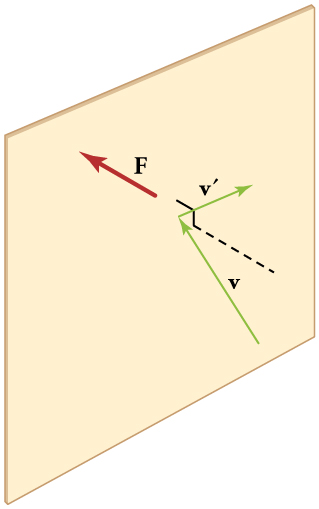
A green vector v, representing a molecule colliding with a wall, is pointing at the surface of a wall at an angle. A second vector v primed starts at the point of impact and travels away from the wall at an angle. A dotted line perpendicular to the wall through the point of impact represents the component of the molecule’s momentum that is perpendicular to the wall. A red vector F is pointing into the wall from the point of impact, representing the force of the molecule hitting the wall.
Figure 13.21 — 13.4 Theory: Atomic and Molecular Explanation of Pressure and Temperature

Figure 13.21 When a molecule collides with a rigid wall, the component of its momentum perpendicular to the wall is reversed. A force is thus exerted on the wall, creating pressure.

Paul Peter Urone and Roger Hinrichs, College Physics 2E, OpenStax. · CC BY-NC-SA 4.0 · Original image ↗ · Access for free ↗
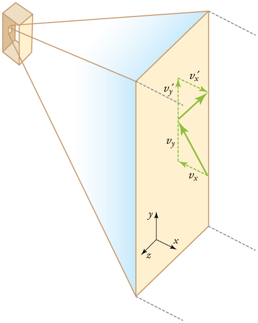
Diagram representing the pressures that a gas exerts on the walls of a box in a three-dimensional coordinate system with x, y, and z components.
Figure 13.22 — 13.4 Theory: Atomic and Molecular Explanation of Pressure and Temperature

Figure 13.22 Gas in a box exerts an outward pressure on its walls. A molecule colliding with a rigid wall has the direction of its velocity and momentum in the x x -direction reversed. This direction is perpendicular to the wall. The components of its velocity momentum in the y y - and z z -directions are not changed, which means there is no force parallel to the wall.

Paul Peter Urone and Roger Hinrichs, College Physics 2E, OpenStax. · CC BY-NC-SA 4.0 · Original image ↗ · Access for free ↗
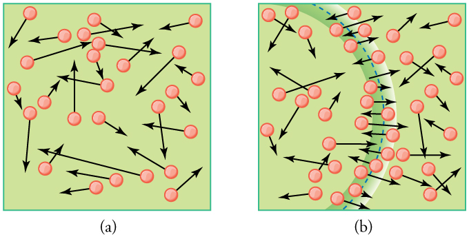
In part a of the figure, circles represent molecules distributed in a gas. Attached to each circle is a vector representing velocity. The circles have a random arrangement, while the vector arrows have random orientations and lengths. In part b of the figure, an arc represents a sound wave as it passes through a gas. The velocity of each molecule along the peak of the wave is roughly oriented parallel to the transmission direction of the wave.
Figure 13.23 — 13.4 Theory: Atomic and Molecular Explanation of Pressure and Temperature

Figure 13.23 (a) There are many molecules moving so fast in an ordinary gas that they collide a billion times every second. (b) Individual molecules do not move very far in a small amount of time, but disturbances like sound waves are transmitted at speeds related to the molecular speeds.

Paul Peter Urone and Roger Hinrichs, College Physics 2E, OpenStax. · CC BY-NC-SA 4.0 · Original image ↗ · Access for free ↗
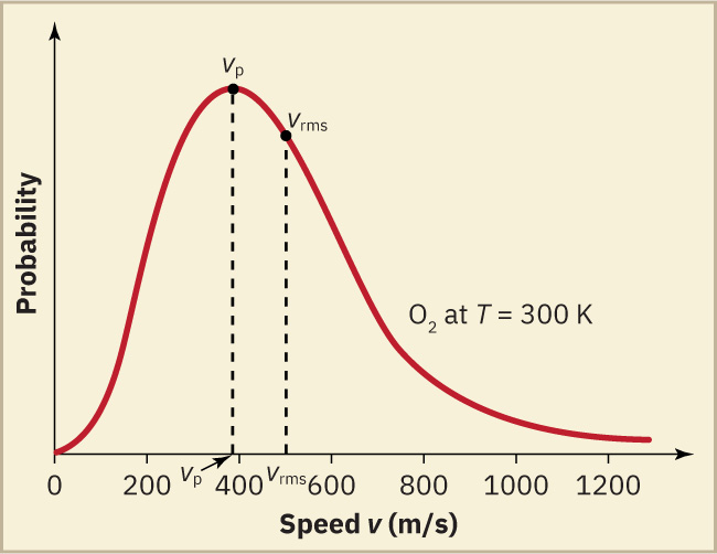
A line graph of probability versus velocity in meters per second of oxygen gas at 300 kelvin. The graph is skewed to the right, with a peak probability just under 400 meters per second and a root-mean-square probability of about 500 meters per second.
Figure 13.24 — 13.4 Theory: Atomic and Molecular Explanation of Pressure and Temperature

Figure 13.24 The Maxwell-Boltzmann distribution of molecular speeds in an ideal gas. The most likely speed v p v p is less than the rms speed v rms v rms . Although very high speeds are possible, only a tiny fraction of the molecules have speeds that are an order of magnitude greater than v rms v rms .

Paul Peter Urone and Roger Hinrichs, College Physics 2E, OpenStax. · CC BY-NC-SA 4.0 · Original image ↗ · Access for free ↗
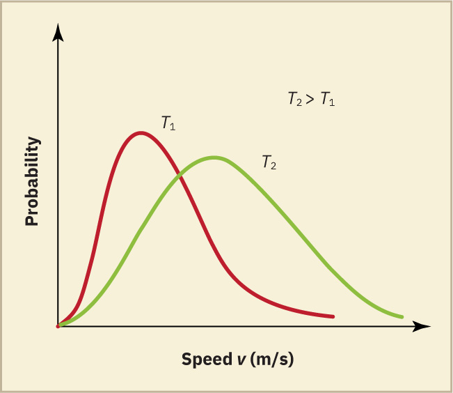
Two distributions of probability versus velocity at two different temperatures plotted on the same graph. Temperature two is greater than Temperature one. The distribution for Temperature two has a peak with a lower probability, but a higher velocity than the distribution for Temperature one. The T sub two graph has a more normal distribution and is broader while the T sub one graph is more narrow and has a tail extending to the right.
Figure 13.25 — 13.4 Theory: Atomic and Molecular Explanation of Pressure and Temperature

Figure 13.25 The Maxwell-Boltzmann distribution is shifted to higher speeds and is broadened at higher temperatures.

Paul Peter Urone and Roger Hinrichs, College Physics 2E, OpenStax. · CC BY-NC-SA 4.0 · Original image ↗ · Access for free ↗
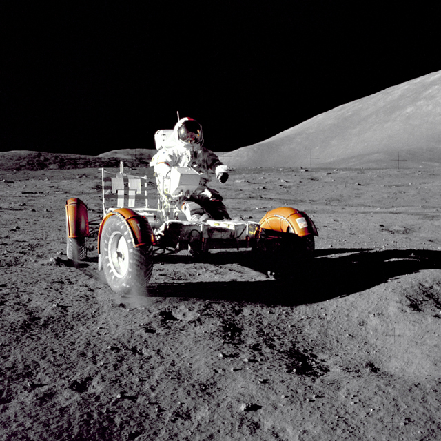
Photograph of the lunar rover on the Moon. The photo looks like it was taken at night with a powerful spotlight shining on the rover from the left: light reflects off the rover, the astronaut, and the Moon’s surface, but the sky is black. The shadow of the rover is very sharp.
Figure 13.26 — 13.4 Theory: Atomic and Molecular Explanation of Pressure and Temperature
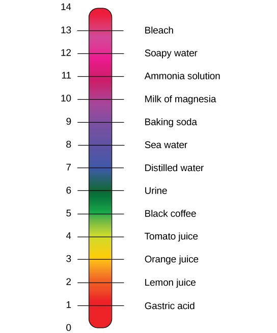
Figure 13.26 This photograph of Apollo 17 Commander Eugene Cernan driving the lunar rover on the Moon in 1972 looks as though it was taken at night with a large spotlight. In fact, the light is coming from the Sun. Because the acceleration due to gravity on the Moon is so low (about 1/6 that of Earth), the Moon’s escape velocity is much smaller. As a result, gas molecules escape very easily from the Moon, leaving it with virtually no atmosphere. Even during the daytime, the sky is black because there is no gas to scatter sunlight. (credit: Harrison H. Schmitt/NASA)

Paul Peter Urone and Roger Hinrichs, College Physics 2E, OpenStax. (credit: Harrison H. Schmitt/NASA) · CC BY-NC-SA 4.0 · Original image ↗ · Access for free ↗

Source: 13.4 Kinetic Theory: Atomic and Molecular Explanation of Pressure and Temperature
145 terms, alphabetically ordered

absolute temperature

temperature measured from absolute zero; gas-law ratios require this scale.

Read explanation · OpenStax ↗
Acid · ·

In the Brønsted–Lowry model, a substance that can donate a . Acidic have a higher activity than water.

Read explanation · OpenStax ↗
Activation energy ·

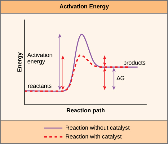
The energy barrier that must overcome to reach a and undergo .

Read explanation · OpenStax ↗
Adenosine triphosphate

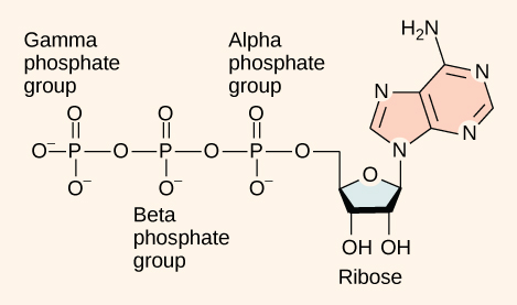
An energy-carrying ; its powers many cellular processes, including cycles.

Read explanation · OpenStax ↗
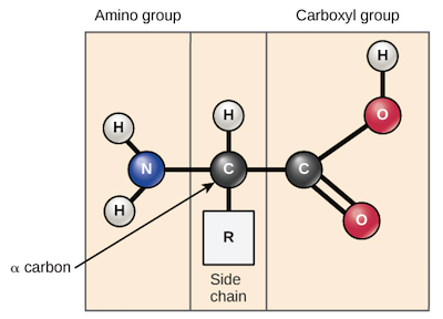
Alpha carbon · ·

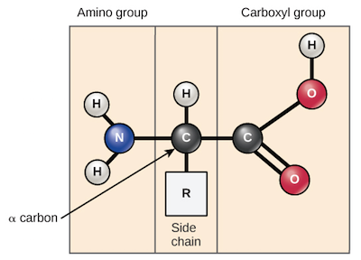
The central carbon next to the carboxyl carbon. In a standard it binds an , hydrogen, and .

Read explanation · OpenStax ↗
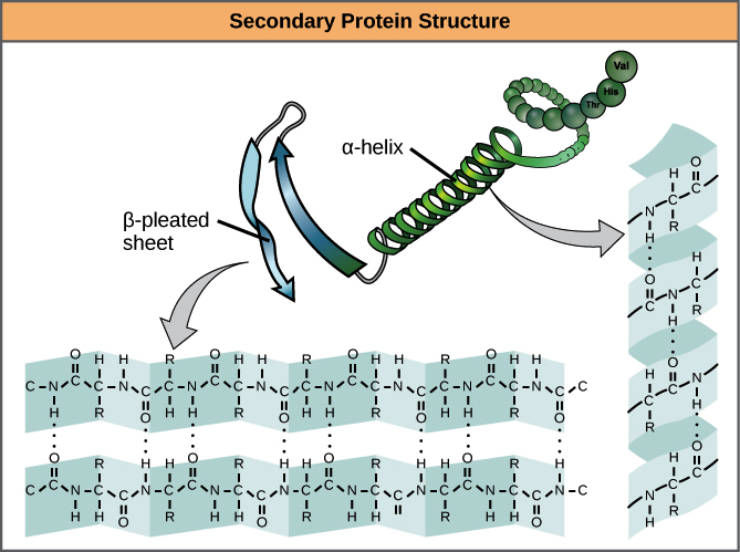
Alpha helix · · · · · ·

A helical stabilized by between a oxygen and an hydrogen four later.

Read explanation · OpenStax ↗
Amide · · ·

A group containing a carbon bonded to nitrogen. are amide linkages.

Read explanation · OpenStax ↗
Amino acid

A building block containing amino and and a characteristic .

Read explanation · OpenStax ↗
Amino acid residue · ·

The part of an incorporated into a chain. Residue can also describe another building block within a larger .

Read explanation · OpenStax ↗
Amino group · · ·

A nitrogen-containing . A free ’s amino group is typically (NH₃⁺) near physiological ; ’s ring nitrogen is an exception to this formula.

Read explanation · OpenStax ↗
Amphipathic

Having both a region and a region, as in a or .

Read explanation · OpenStax ↗
Analytical standard ·

A material with a known identity or amount used to compare or calibrate measurements.

Read explanation · Agilent ↗
Antiparallel

Running in opposite directions, as with two strands or neighboring strands in some .

Read explanation · OpenStax ↗
Aqueous solution ·

A in which water is the .

Read explanation · OpenStax ↗
Aromatic

Containing a cyclic, with . , , and have aromatic .

Read explanation · OpenStax ↗
Atom

The smallest unit of an element that retains its chemical identity; it has a surrounded by .

Read explanation · OpenStax ↗
base dissociation constant

for a ’s with water to form its and hydroxide.

Read explanation · OpenStax ↗
Benzene ring

A six-carbon ring with .

Read explanation · OpenStax ↗
Benzyl group

A attached through a –CH₂– group; part of ’s .

Read explanation · OpenStax ↗
Beta sheet · · · · · ·

A made of aligned segments connected by ; strands may be parallel or .

Read explanation · OpenStax ↗
Biomolecule

A made by or involved in living systems, including , , , and .

Read explanation · OpenStax ↗
Blotting ·

Transfer of separated or to a so a specific target can be detected.

Read explanation · Thermo Fisher ↗
Boltzmann constant

Constant = R/NA connecting temperature with energy per particle.

Read explanation · OpenStax ↗
Brønsted–Lowry base · · · · · · · · · · ·

In the Brønsted–Lowry model, a substance that can accept a . Basic solutions have lower activity than water.

Read explanation · OpenStax ↗
Calibration

Establishing the relation between a measured signal and known values or .

Read explanation · Agilent ↗
Carbohydrate

A class of including sugars and their , used for energy storage, structure, and recognition.

Read explanation · OpenStax ↗
Carbonyl group · ·

A carbon double-bonded to oxygen, C=O; present in and many other .

Read explanation · OpenStax ↗
Carboxyl group · ·

An , COOH. In free it is usually to COO⁻ near physiological .

Read explanation · OpenStax ↗
Catalyst · ·

A substance that speeds a by providing a pathway with lower and is regenerated rather than consumed overall.

Read explanation · OpenStax ↗
Chemical compound ·

A substance containing of two or more different chemically combined in a definite composition.

Read explanation · OpenStax ↗
Chemical element

A substance defined by having the same number of , such as carbon or oxygen.

Read explanation · OpenStax ↗
Chemical reaction ·

A process that rearranges and chemical bonds, converting into .

Read explanation · OpenStax ↗
Chromatin

The complex of and associated , including , in .

Read explanation · OpenStax ↗
Chromatographic peak · ·

A rise and fall in detector signal as one or more components pass through the detector; a peak does not guarantee a single pure .

Read explanation · Agilent ↗
Chromosome ·

An organized with associated that carries . A replicated chromosome has two .

Read explanation · OpenStax ↗
Codon

A sequence of three that specifies an or a stop signal.

Read explanation · OpenStax ↗
compressibility factor

Dimensionless ratio PV/(nRT), equal to one for an .

Read explanation · OpenStax ↗
Concentration

The amount of a substance in a specified volume or mass of mixture.

Read explanation · OpenStax ↗
conjugate acid

Species formed when a gains one .

Read explanation · OpenStax ↗
Conjugated system ·

Adjacent orbitals that allow to be distributed across several , often through alternating single and multiple bonds.

Read explanation · OpenStax ↗
Covalent bond · ·

A bond in which share pairs. and are covalent.

Read explanation · OpenStax ↗
Cysteine ·

An with a . Two cysteines can form a .

Read explanation · OpenStax ↗
Dalton

A unit of mass equal to one twelfth of the mass of a carbon-12 ; used to describe .

Read explanation · OpenStax ↗
Dalton’s law

The total pressure of an mixture equals the sum of component partial pressures.

Read explanation · OpenStax ↗
Deoxyribonucleic acid

The that stores genetic information used to specify and sequences.

Read explanation · OpenStax ↗
Deprotonation

Removal of a from a or group; this changes its by minus one.

Read explanation · OpenStax ↗
Detergent

An substance that can associate with both water and material; detergents can disrupt or interactions.

Read explanation · Thermo Fisher ↗
Disulfide bond · · ·

A covalent sulfur–sulfur bond formed by of two , which can stabilize structure.

Read explanation · NCBI Bookshelf ↗
DNA replication

Copying so genetic information can be passed to daughter cells. Each guides a complementary new strand.

Read explanation · OpenStax ↗
Electric charge · · ·

An electrical property that can be positive or negative. Opposite charges attract and like charges repel; net charge is the sum of all charges on a particle.

Read explanation · OpenStax ↗
Electron

A negatively subatomic particle. Electron sharing and transfer determine much of chemical bonding.

Read explanation · OpenStax ↗
Electron delocalization ·

Distribution of across several rather than confinement to one or bond.

Read explanation · OpenStax ↗
Electronegativity ·

An ’s tendency to attract shared in a chemical bond. Unequal attraction can make a bond .

Read explanation · OpenStax ↗
Entropy

A measure related to the number of accessible microscopic arrangements and the dispersal of energy.

Read explanation · OpenStax ↗
Equilibrium

A state where opposing processes occur at equal rates, so macroscopic or other properties remain constant.

Read explanation · OpenStax ↗
Equilibrium constant

A ratio of to activities at , each raised to its stoichiometric coefficient. At a fixed temperature, a does not change this ratio.

Read explanation · OpenStax ↗
Eukaryote ·

An organism whose cells have a -enclosed ; animals, plants, fungi, and protists are eukaryotes.

Read explanation · OpenStax ↗
FACT complex ·

A -associated complex that helps machinery traverse and supports reorganization.

Read explanation · OpenStax ↗
Fraction · ·

A portion of a sample collected during a separation, such as the fluid leaving a column during a time interval.

Read explanation · Waters ↗
Functional group

A group of whose chemical behavior gives a characteristic and properties.

Read explanation · OpenStax ↗
Gene

A sequence that contributes to a functional or , together with the information needed to express it.

Read explanation · OpenStax ↗
Gene expression

Production of a functional from a , including and, for -coding , .

Read explanation · NCBI Bookshelf ↗
heat capacity

Heat required per temperature change under specified conditions.

Read explanation · OpenStax ↗
Histidine ·

A with an . Mostly uncharged near physiological , it can accept or donate .

Read explanation · OpenStax ↗
Histone

A -associated rich in . Core histones form the around which nucleosomal wraps.

Read explanation · OpenStax ↗
Hydrogen bond ·

An attraction between a hydrogen bonded to an and another . hydrogen bonds stabilize .

Read explanation · OpenStax ↗
Hydrogen ion · ·

A positively hydrogen species. H⁺ denotes a , which is hydrated in water; its activity determines .

Read explanation · OpenStax ↗
Hydrolysis

Breaking a chemical bond by adding water. hydrolysis separates .

Read explanation · OpenStax ↗
Hydrophilic

Interacting favorably with water, typically because a group is or .

Read explanation · OpenStax ↗
Hydrophobic

Interacting poorly with water. often gather in a ’s interior.

Read explanation · OpenStax ↗
Hydroxide ion ·

The negatively OH⁻. Basic contain a higher hydroxide ion activity than water at the same temperature.

Read explanation · OpenStax ↗
Hydroxyl group ·

An oxygen bonded to hydrogen, –OH. Hydroxyl groups can and often increase .

Read explanation · OpenStax ↗
ideal gas

Model gas with negligible particle volume and negligible intermolecular interactions.

Read explanation · OpenStax ↗
Imidazole

A five-membered ring containing two nitrogens; ’s contains this ring.

Read explanation · OpenStax ↗
Indole

A fused six-membered and five-membered ring system containing nitrogen; found in .

Read explanation · OpenStax ↗
internal energy

Total microscopic energy within a system under a specified description.

Read explanation · OpenStax ↗
Ion · ·

An or with a net because its numbers of and do not balance.

Read explanation · OpenStax ↗
Kinetic energy

Energy associated with motion; higher temperature generally increases average molecular kinetic energy.

Read explanation · OpenStax ↗
Kinetics

The study of and the factors and mechanisms that control them. A favorable may still proceed slowly.

Read explanation · OpenStax ↗
linkage

A tendency of nearby on the same to be inherited together.

Read explanation · OpenStax ↗
Lipid

A broad class of largely or , including fats, , and steroids.

Read explanation · OpenStax ↗
locus

The specific position of a or other feature.

Read explanation · OpenStax ↗
Logarithm · · ·

The exponent needed to obtain a number from a chosen fixed number. For decimal logarithms, log₁₀(100) = 2 because 10² = 100; uses the negative decimal logarithm of activity.

Read explanation · OpenStax ↗
mechanical power

Rate of energy transfer, measured in watts.

Read explanation · OpenStax ↗
mechanical work

Energy transferred by a force acting through ; the force component parallel to motion contributes.

Read explanation · OpenStax ↗
Membrane · · · ·

A thin boundary or sheet. Cell membranes are bilayers containing ; membranes are synthetic supports that hold or for detection.

Read explanation · OpenStax ↗
Messenger RNA ·

An that carries coding information used by to synthesize a .

Read explanation · OpenStax ↗
molar mass

Mass per of a specified substance.

Read explanation · OpenStax ↗
mole

Amount containing exactly 6.02214076 × 10²³ specified entities.

Read explanation · OpenStax ↗
Molecular chaperone · ·

A that assists other in folding or prevents , without specifying their sequence.

Read explanation · NCBI Bookshelf ↗
molecular formula

Actual number of each type of in a .

Read explanation · OpenStax ↗
Molecular mass · ·

The mass of a , commonly expressed in for . Molecular weight is often used informally for the same quantity.

Read explanation · OpenStax ↗
Molecule

Two or more joined by . A molecule may be electrically or carry a .

Read explanation · OpenStax ↗
Neutral

Having no net . For a , neutral instead means equal and activities; its is about 7 at 25 °C.

Read explanation · OpenStax ↗
Nitrogenous base · · ·

A nitrogen-containing ring component of ; its pairing interactions help specify sequences.

Read explanation · OpenStax ↗
Nonpolar ·

Lacking a substantial separation of . Nonpolar groups generally interact poorly with water.

Read explanation · OpenStax ↗
Nucleic acid

A of , such as or , used in information storage, expression, and other cellular functions.

Read explanation · OpenStax ↗
Nucleosome

The basic unit of : wrapped around a .

Read explanation · OpenStax ↗
Nucleotide

A joined to a sugar and one or more .

Read explanation · OpenStax ↗
Nucleus ·

A -enclosed compartment containing most of a cell’s .

Read explanation · OpenStax ↗
Octamer

A complex made of eight . A core contains eight .

Read explanation · OpenStax ↗
Oxidation ·

Loss of or an increase in oxidation state. Oxidizing two can form a .

Read explanation · OpenStax ↗
Peptide

A chain of joined by ; the term commonly describes chains shorter than a typical .

Read explanation · OpenStax ↗
Peptide bond ·

A covalent between the carboxyl carbon of one and the amino nitrogen of the next.

Read explanation · OpenStax ↗
pH

A measure of , defined as the negative of activity. Lower pH means greater ; pH influences .

Read explanation · OpenStax ↗
Phenylalanine ·

A with an .

Read explanation · OpenStax ↗
Phosphate group ·

A phosphorus-containing group bonded to oxygens; phosphate groups occur in , , and modified .

Read explanation · OpenStax ↗
Phospholipid

An with a -containing region and tails; a major component of cellular .

Read explanation · OpenStax ↗
physical displacement ·

Signed or difference between final and initial position.

Read explanation · OpenStax ↗
Polar

Having an uneven distribution of . Polar groups often interact favorably with water.

Read explanation · OpenStax ↗
Polymer

A large made from many linked molecular building blocks.

Read explanation · OpenStax ↗
Polypeptide

A chain of connected by . A functional can contain one or several such chains.

Read explanation · OpenStax ↗
Proline ·

An whose loops back to the nitrogen, restricting rotation and often creating bends.

Read explanation · OpenStax ↗
Protein

One or more folded chains that perform biological roles such as , transport, signaling, or structural support.

Read explanation · OpenStax ↗
Protein aggregation · ·

Association of into larger clusters, often when exposed surfaces of unfolded stick together.

Read explanation · NCBI Bookshelf ↗
Protein backbone ·

The repeating nitrogen–alpha-carbon– chain of a , excluding its variable .

Read explanation · OpenStax ↗
Proton

A positively subatomic particle. In – chemistry, donating a proton means transferring a .

Read explanation · OpenStax ↗
Protonation

Addition of a to an , , or ; this changes its by plus one.

Read explanation · OpenStax ↗
Quantification · ·

Estimating the amount or of a substance from measured signals and suitable or .

Read explanation · Waters ↗
R group · ·

The variable side chain attached to an ’s . It determines identity, , , and chemical behavior.

Read explanation · OpenStax ↗
Reactant

A starting substance transformed during a .

Read explanation · OpenStax ↗
Reaction intermediate · ·

A species formed in one step and consumed in another. It occupies a local energy minimum between .

Read explanation · OpenStax ↗
Reaction product ·

A substance formed by a .

Read explanation · OpenStax ↗
Reaction rate · ·

How quickly are consumed or form, usually expressed as a change per unit time.

Read explanation · OpenStax ↗
Ribonucleic acid ·

A with roles in , regulation, and ; carries -coding information.

Read explanation · OpenStax ↗
Ribosome ·

A complex of and that translates into a .

Read explanation · OpenStax ↗
root-mean-square speed

Square root of the mean squared particle speed; for an it is √(3RT/M).

Read explanation · OpenStax ↗
Secondary structure

Local folding, such as and , stabilized mainly by .

Read explanation · OpenStax ↗
Sister chromatid

One of the two copies of a produced by . An intact sister chromatid can supply a template for accurate repair.

Read explanation · Biology LibreTexts / Oregon State University ↗
Solubility ·

The amount of a substance that can dissolve in a under specified conditions. Soluble means able to dissolve; insoluble means only very slightly soluble in that .

Read explanation · OpenStax ↗
Solute

A dissolved component of a .

Read explanation · OpenStax ↗
Solution

A homogeneous mixture in which are dissolved in a .

Read explanation · OpenStax ↗
Solvent

The component of a that dissolves other substances, usually the component present in the greatest amount.

Read explanation · OpenStax ↗
spatial vector ·

Quantity with both magnitude and direction, combined by adding components.

Read explanation · OpenStax ↗
Subunit ·

An individual chain within a containing multiple chains.

Read explanation · OpenStax ↗
Template strand · · ·

A preexisting strand whose sequence guides complementary nucleic- synthesis.

Read explanation · OpenStax ↗
Thermodynamics ·

The study of energy, , and . It helps determine whether a process is favorable, while concerns how fast it occurs.

Read explanation · OpenStax ↗
Thiol group · · · ·

A sulfur bonded to hydrogen, –SH. thiols can form through .

Read explanation · OpenStax ↗
Transcription

Synthesis of using a template.

Read explanation · OpenStax ↗
Transition state

A fleeting, high-energy arrangement at a barrier. It is an energy maximum along the path, rather than a stable .

Read explanation · OpenStax ↗
Translation ·

Synthesis of a on a using the sequence of in .

Read explanation · OpenStax ↗
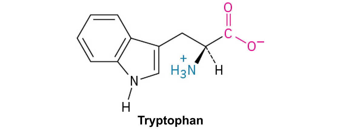
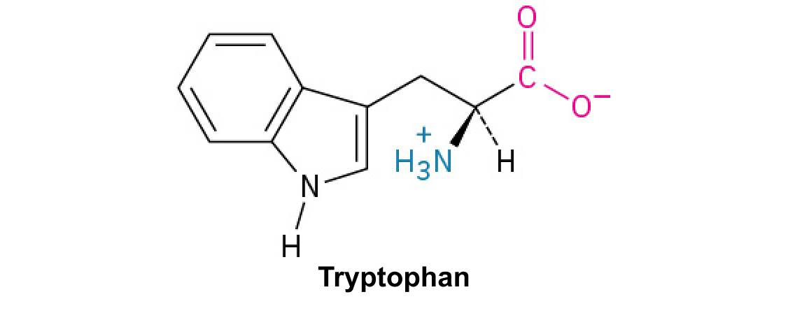
Tryptophan ·

An with a bulky ; commonly grouped as .

Read explanation · OpenStax ↗
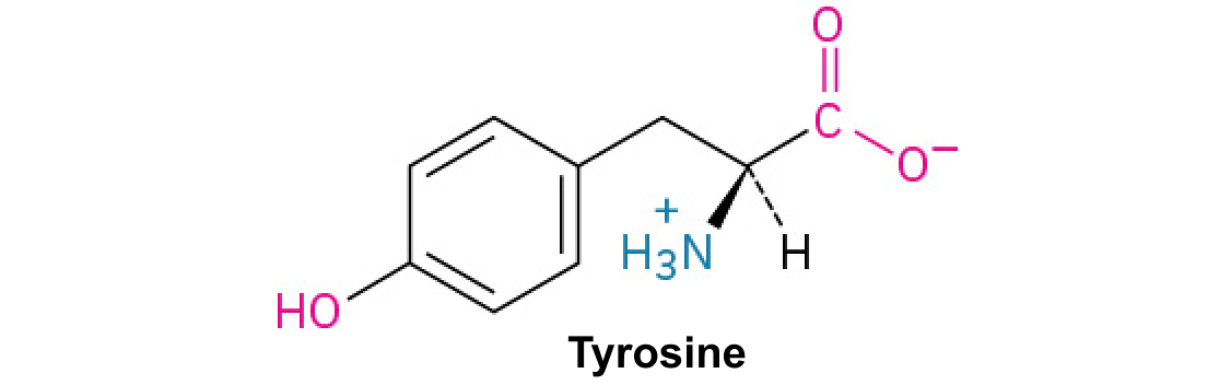
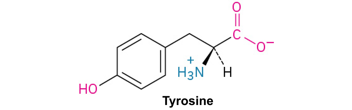
Tyrosine ·

An with a phenolic . Usually uncharged near physiological .

Read explanation · OpenStax ↗
van der Waals equation

Real-gas model correcting ideal pressure for attractions and ideal volume for particle size.

Read explanation · OpenStax ↗
velocity

Rate of change of position, including direction.

Read explanation · OpenStax ↗

9.5 The Kinetic-Molecular Theory

OpenStax · 9.5 The Kinetic-Molecular Theory ↗
Instructional page including learning objectives, examples, figures, source tables and questions. Site navigation and embedded media players are omitted; source media links remain available.

Learning Objectives

  • State the postulates of the -molecular theory
  • Use this theory’s postulates to explain the gas laws

The gas laws that we have seen to this point, as well as the equation, are empirical, that is, they have been derived from experimental observations. The mathematical forms of these laws closely describe the macroscopic behavior of most gases at pressures less than about 1 or 2 atm. Although the gas laws describe relationships that have been verified by many experiments, they do not tell us why gases follow these relationships.

The molecular theory (KMT) is a simple microscopic model that effectively explains the gas laws described in previous modules of this chapter. This theory is based on the following five postulates described here. (Note: The term “” will be used to refer to the individual chemical species that compose the gas, although some gases are composed of atomic species, for example, the noble gases.)

  1. Gases are composed of that are in continuous motion, travelling in straight lines and changing direction only when they collide with other or with the walls of a container.
  2. The composing the gas are negligibly small compared to the distances between them.
  3. The pressure exerted by a gas in a container results from collisions between the gas and the container walls.
  4. Gas exert no attractive or repulsive forces on each other or the container walls; therefore, their collisions are elastic (do not involve a loss of energy).
  5. The average of the gas is proportional to the temperature of the gas.

The test of the KMT and its postulates is its ability to explain and describe the behavior of a gas. The various gas laws can be derived from the assumptions of the KMT, which have led chemists to believe that the assumptions of the theory accurately represent the properties of gas . We will first look at the individual gas laws (Boyle’s, Charles’s, Amontons’s, Avogadro’s, and ’s laws) conceptually to see how the KMT explains them. Then, we will more carefully consider the relationships between , speeds, and energies with temperature, and explain Graham’s law.

The -Molecular Theory Explains the Behavior of Gases, Part I

Recalling that gas pressure is exerted by rapidly moving gas and depends directly on the number of hitting a unit area of the wall per unit of time, we see that the KMT conceptually explains the behavior of a gas as follows:

  • Amontons’s law. If the temperature is increased, the average speed and of the gas increase. If the volume is held constant, the increased speed of the gas results in more frequent and more forceful collisions with the walls of the container, therefore increasing the pressure (Figure 9.31).
  • Charles’s law. If the temperature of a gas is increased, a constant pressure may be maintained only if the volume occupied by the gas increases. This will result in greater average distances traveled by the to reach the container walls, as well as increased wall surface area. These conditions will decrease both the frequency of -wall collisions and the number of collisions per unit area, the combined effects of which balance the effect of increased collision forces due to the greater at the higher temperature.
  • Boyle’s law. If the gas volume of a given amount of gas at a given temperature is decreased (that is, if the gas is compressed), the will be exposed to a decreased container wall area. Collisions with the container wall will therefore occur more frequently and the pressure exerted by the gas will increase (Figure 9.31).
  • Avogadro’s law. At constant pressure and temperature, the frequency and force of -wall collisions are constant. Under such conditions, increasing the number of gaseous will require a proportional increase in the container volume in order to yield a decrease in the number of collisions per unit area to compensate for the increased frequency of collisions (Figure 9.31).
  • . Because of the large distances between them, the of one gas in a mixture bombard the container walls with the same frequency whether other gases are present or not, and the total pressure of a gas mixture equals the sum of the (partial) pressures of the individual gases.
This figure shows 3 pairs of pistons and cylinders. In a, which is labeled, “Charles’s Law,” the piston is positioned for the first cylinder so that just over half of the available volume contains 6 purple spheres with trails behind them. The trails indicate movement. Orange dashes extend from the interior surface of the cylinder where the spheres have collided. This cylinder is labeled, “Baseline.” In the second cylinder, the piston is in the same position, and the label, “Heat” is indicated in red capitalized text. Four red arrows with wavy stems are pointing upward to the base of the cylinder. The six purple spheres have longer trails behind them and the number of orange dashes indicating points of collision with the container walls has increased. A rectangle beneath the diagram states, “Temperature increased, Volume constant equals Increased pressure.” In b, which is labeled, “Boyle’s Law,” the first, baseline cylinder shown is identical to the first cylinder in a. In the second cylinder, the piston has been moved, decreasing the volume available to the 6 purple spheres to half of the initial volume. The orange dashes indicating points of collision with the container walls has increased. This second cylinder is labeled, “Volume decreased.” A rectangle beneath the diagram states, “Volume decreased, Wall area decreased equals Increased pressure.” In c, which is labeled “Avogadro’s Law,” the first, baseline cylinder shown is identical to the first cylinder in a. In the second cylinder, the number of purple spheres has changed from 6 to 12 and volume has doubled. This second cylinder is labeled “Increased gas.” A rectangle beneath the diagram states, “At constant pressure, More gas molecules added equals Increased volume.”
Figure 9.31 — 9.5 The -Molecular Theory

Figure 9.31 (a) When gas temperature increases, gas pressure increases due to increased force and frequency of molecular collisions. (b) When volume decreases, gas pressure increases due to increased frequency of molecular collisions. (c) When the amount of gas increases at a constant pressure, volume increases to yield a constant number of collisions per unit wall area per unit time.

Paul Flowers, Klaus Theopold, Richard Langley, and William R. Robinson, Chemistry 2E, OpenStax. · CC BY-NC-SA 4.0 · Original image ↗ · Access for free ↗

Molecular Speeds and

The previous discussion showed that the KMT qualitatively explains the behaviors described by the various gas laws. The postulates of this theory may be applied in a more fashion to derive these individual laws. To do this, we must first look at speeds and energies of gas , and the temperature of a gas sample.

In a gas sample, individual have widely varying speeds; however, because of the vast number of and collisions involved, the molecular speed distribution and average speed are constant. This molecular speed distribution is known as a Maxwell-Boltzmann distribution, and it depicts the relative numbers of in a bulk sample of gas that possesses a given speed (Figure 9.32).

A graph is shown. The horizontal axis is labeled, “Speed u ( m divided by s ).” This axis is marked by increments of 20 beginning at 0 and extending up to 120. The vertical axis is labeled, “Fraction of molecules.” A positively or right-skewed curve is shown in red which begins at the origin and approaches the horizontal axis around 120 m per s. At the peak of the curve, a point is indicated with a black dot and is labeled, “v subscript p.” A vertical dashed line extends from this point to the horizontal axis at which point the intersection is labeled, “v subscript p.” Slightly to the right of the peak a second black dot is placed on the curve. This point is labeled, “v subscript r m s.” A vertical dashed line extends from this point to the horizontal axis at which point the intersection is labeled, “v subscript r m s.” The label, “O subscript 2 at T equals 300 K” appears in the open space to the right of the curve.
Figure 9.32 — 9.5 The -Molecular Theory

Figure 9.32 The molecular speed distribution for oxygen gas at 300 K is shown here. Very few molecules move at either very low or very high speeds. The number of molecules with intermediate speeds increases rapidly up to a maximum, which is the most probable speed, then drops off rapidly. Note that the most probable speed, ν p , is a little less than 400 m/s, while the root mean square speed, u rms , is closer to 500 m/s.

Paul Flowers, Klaus Theopold, Richard Langley, and William R. Robinson, Chemistry 2E, OpenStax. · CC BY-NC-SA 4.0 · Original image ↗ · Access for free ↗

The (KE) of a particle of mass (m) and speed (u) is given by:

KE=12mu2

Expressing mass in kilograms and speed in meters per second will yield energy values in units of joules (J = kg m2 s–2). To deal with a large number of gas , we use averages for both speed and . In the KMT, the root mean square speed of a particle, urms, is defined as the square root of the average of the squares of the speeds with n = the number of particles:

urms=u2¯=u12+u22+u32+u42+…n

The average for a of particles, KEavg, is then equal to:

KEavg=12Murms2

where M is the expressed in units of kg/mol. The KEavg of a of gas is also directly proportional to the temperature of the gas and may be described by the equation:

KEavg=32RT

where R is the gas constant and T is the temperature. When used in this equation, the appropriate form of the gas constant is 8.314 J/mol⋅K (8.314 kg m2s–2mol–1K–1). These two separate equations for KEavg may be combined and rearranged to yield a relation between molecular speed and temperature:

12Murms2=32RT
urms=3RTM

Example 9.23

Calculation of urms

Calculate the for a nitrogen at 30 °C.

Convert the temperature into :
30°C+273=303 K

Determine the of nitrogen in kilograms:

28.0g1 mol×1 kg1000g=0.028kg/mol

Replace the variables and constants in the equation, replacing Joules with the equivalent kg m2s–2:

urms=3RTM
urms=3(8.314J/mol K)(303 K)(0.028kg/mol)=2.70×105m2s−2=519m/s

Check Your Learning

Calculate the for a of oxygen at –23 °C.

Answer:

441 m/s

If the temperature of a gas increases, its KEavg increases, more have higher speeds and fewer have lower speeds, and the distribution shifts toward higher speeds overall, that is, to the right. If temperature decreases, KEavg decreases, more have lower speeds and fewer have higher speeds, and the distribution shifts toward lower speeds overall, that is, to the left. This behavior is illustrated for nitrogen gas in Figure 9.33.

A graph with four positively or right-skewed curves of varying heights is shown. The horizontal axis is labeled, “Speed u ( m divided by s ).” This axis is marked by increments of 500 beginning at 0 and extending up to 1500. The vertical axis is labeled, “Fraction of molecules.” The label, “N subscript 2,” appears in the open space in the upper right area of the graph. The tallest and narrowest of these curves is labeled, “100 K.” Its right end appears to touch the horizontal axis around 700 m per s. It is followed by a slightly wider curve which is labeled, “200 K,” that is about three quarters of the height of the initial curve. Its right end appears to touch the horizontal axis around 850 m per s. The third curve is significantly wider and only about half the height of the initial curve. It is labeled, “500 K.” Its right end appears to touch the horizontal axis around 1450 m per s. The final curve is only about one third the height of the initial curve. It is much wider than the others, so much so that its right end has not yet reached the horizontal axis. This curve is labeled, “1000 K.”
Figure 9.33 — 9.5 The -Molecular Theory

Figure 9.33 The molecular speed distribution for nitrogen gas (N 2 ) shifts to the right and flattens as the temperature increases; it shifts to the left and heightens as the temperature decreases.

Paul Flowers, Klaus Theopold, Richard Langley, and William R. Robinson, Chemistry 2E, OpenStax. · CC BY-NC-SA 4.0 · Original image ↗ · Access for free ↗

At a given temperature, all gases have the same KEavg for their . Gases composed of lighter have more high-speed particles and a higher urms, with a speed distribution that at relatively higher speeds. Gases consisting of heavier have more low-speed particles, a lower urms, and a speed distribution that at relatively lower speeds. This trend is demonstrated by the data for a series of noble gases shown in Figure 9.34.

A graph is shown with four positively or right-skewed curves of varying heights. The horizontal axis is labeled, “Speed u ( m divided by s ).” This axis is marked by increments of 500 beginning at 0 and extending up to 3000. The vertical axis is labeled, “Fraction of molecules.” The tallest and narrowest of these curves is labeled, “X e.” Its right end appears to touch the horizontal axis around 600 m per s. It is followed by a slightly wider curve which is labeled, “A r,” that is about half the height of the initial curve. Its right end appears to touch the horizontal axis around 900 m per s. The third curve is significantly wider and just over a third of the height of the initial curve. It is labeled, “N e.” Its right end appears to touch the horizontal axis around 1200 m per s. The final curve is only about one fourth the height of the initial curve. It is much wider than the others, so much so that its right reaches the horizontal axis around 2500 m per s. This curve is labeled, “H e.”
Figure 9.34 — 9.5 The -Molecular Theory

Figure 9.34 molecular speed is directly related to molecular mass. At a given temperature, lighter molecules move faster on average than heavier molecules.

Paul Flowers, Klaus Theopold, Richard Langley, and William R. Robinson, Chemistry 2E, OpenStax. · CC BY-NC-SA 4.0 · Original image ↗ · Access for free ↗

Link to Learning

The gas simulator may be used to examine the effect of temperature on molecular speeds. Examine the simulator’s “energy histograms” (molecular speed distributions) and “species information” (which gives average speed values) for of different masses at various temperatures.

The -Molecular Theory Explains the Behavior of Gases, Part II

According to Graham’s law, the of a gas are in rapid motion and the themselves are small. The average distance between the of a gas is large compared to the size of the . As a consequence, gas can move past each other easily and diffuse at relatively fast rates.

The rate of effusion of a gas depends directly on the (average) speed of its :

effusion rate∝urms

Using this relation, and the equation relating molecular speed to mass, Graham’s law may be easily derived as shown here:

urms=3RTM
M=3RTurms2=3RTu¯2
effusion rate Aeffusion rate B=urmsAurmsB=3RTMA3RTMB=MBMA

The ratio of the rates of effusion is thus derived to be inversely proportional to the ratio of the square roots of their masses. This is the same relation observed experimentally and expressed as Graham’s law.

9.6 Non-Ideal Gas Behavior

OpenStax · 9.6 Non-Ideal Gas Behavior ↗
Instructional page including learning objectives, examples, figures, source tables and questions. Site navigation and embedded media players are omitted; source media links remain available.

Learning Objectives

By the end of this section, you will be able to:

  • Describe the physical factors that lead to deviations from behavior
  • Explain how these factors are represented in the
  • Define compressibility (Z) and describe how its variation with pressure reflects non-ideal behavior
  • non-ideal behavior by comparing computations of gas properties using the law and the

Thus far, the law, PV = nRT, has been applied to a variety of different types of problems, ranging from stoichiometry and empirical and problems to determining the density and of a gas. As mentioned in the previous modules of this chapter, however, the behavior of a gas is often non-ideal, meaning that the observed relationships between its pressure, volume, and temperature are not accurately described by the gas laws. In this section, the reasons for these deviations from behavior are considered.

One way in which the accuracy of PV = nRT can be judged is by comparing the actual volume of 1 of gas (its molar volume, Vm) to the molar volume of an at the same temperature and pressure. This ratio is called the (Z) with:

Z=molar volume of gas at sameTandPmolar volume of ideal gas at sameTandP=(PVmRT)measured

behavior is therefore indicated when this ratio is equal to 1, and any deviation from 1 is an indication of non-ideal behavior. Figure 9.35 shows plots of Z over a large pressure range for several common gases.

A graph is shown. The horizontal axis is labeled, “P ( a t m ).” Its scale begins at zero with markings provided by multiples of 200 up to 1000. The vertical axis is labeled, “Z le( k P a ).” This scale begins at zero and includes multiples of 0.5 up to 2.0. Six curves are drawn of varying colors. One of these curves is a horizontal, light purple line extending right from 1.0 k P a on the vertical axis, which is labeled “Ideal gas.” The region of the graph beneath this line is shaded tan. The remaining curves also start at the same point on the vertical axis. An orange line extends to the upper right corner of the graph, reaching a value of approximately 1.7 k P a at 1000 a t m. This orange curve is labeled, “H subscript 2.” A blue curve dips below the horizontal ideal gas line initially, then increases to cross the line just past 200 a t m. This curve reaches a value of nearly 2.0 k P a at about 800 a t m. This curve is labeled, “N subscript 2.” A red curve dips below the horizontal ideal gas line initially, then increases to cross the line just past 400 a t m. This curve reaches a value of nearly 1.5 k P a at about 750 a t m. This curve is labeled, “O subscript 2.” A purple curve dips below the horizontal ideal gas line, dipping even lower than the O subscript 2 curve initially, then increases to cross the ideal gas line at about 400 a t m. This curve reaches a value of nearly 2.0 k P a at about 850 a t m. This curve is labeled, “C H subscript 4.” A yellow curve dips below the horizontal ideal gas line, dipping lower than the other curves to a minimum of about 0.4 k P a at about 0.75 a t m, then increases to cross the ideal gas line at about 500 a t m. This curve reaches a value of about 1.6 k P a at about 900 a t m. This curve is labeled, “C O subscript 2.”
Figure 9.35 — 9.6 Non- Behavior

Figure 9.35 A graph of the compressibility factor (Z) vs. pressure shows that gases can exhibit significant deviations from the behavior predicted by the ideal gas law.

Paul Flowers, Klaus Theopold, Richard Langley, and William R. Robinson, Chemistry 2E, OpenStax. · CC BY-NC-SA 4.0 · Original image ↗ · Access for free ↗

As is apparent from Figure 9.35, the law does not describe gas behavior well at relatively high pressures. To determine why this is, consider the differences between real gas properties and what is expected of a hypothetical .

Particles of a hypothetical have no significant volume and do not attract or repel each other. In general, real gases approximate this behavior at relatively low pressures and high temperatures. However, at high pressures, the of a gas are crowded closer together, and the amount of empty space between the is reduced. At these higher pressures, the volume of the gas themselves becomes appreciable relative to the total volume occupied by the gas. The gas therefore becomes less compressible at these high pressures, and although its volume continues to decrease with increasing pressure, this decrease is not proportional as predicted by Boyle’s law.

At relatively low pressures, gas have practically no attraction for one another because they are (on average) so far apart, and they behave almost like particles of an . At higher pressures, however, the force of attraction is also no longer insignificant. This force pulls the a little closer together, slightly decreasing the pressure (if the volume is constant) or decreasing the volume (at constant pressure) (Figure 9.36). This change is more pronounced at low temperatures because the have lower KE relative to the attractive forces, and so they are less effective in overcoming these attractions after colliding with one another.

This figure includes two diagrams. Each involves two lavender shaded boxes that contain 14 relatively evenly distributed, purple spheres. The first box in a on the left is labeled “ideal.” In the second slightly smaller box, on the right, a nearly centrally located purple sphere has 6 double-headed arrows extending outward from it to nearby spheres. This box is labeled “real.” In b, in the first box on the left, a single arrow points to a purple sphere at the right side that appears to be moving and impacting the right side of the box. There are no other spheres positioned near the right edge. This box is labeled “ideal.” The second box, on the right, shows the same image but has 5 double-headed arrows radiating out to the top, bottom, and left to other spheres. This box is labeled “real.”
Figure 9.36 — 9.6 Non- Behavior

Figure 9.36 (a) Attractions between gas molecules serve to decrease the gas volume at constant pressure compared to an ideal gas whose molecules experience no attractive forces. (b) These attractive forces will decrease the force of collisions between the molecules and container walls, therefore reducing the pressure exerted at constant volume compared to an ideal gas.

Paul Flowers, Klaus Theopold, Richard Langley, and William R. Robinson, Chemistry 2E, OpenStax. · CC BY-NC-SA 4.0 · Original image ↗ · Access for free ↗

There are several different equations that better approximate gas behavior than does the law. The first, and simplest, of these was developed by the Dutch scientist Johannes van der Waals in 1879. The improves upon the law by adding two terms: one to account for the volume of the gas and another for the attractive forces between them.

The constant a corresponds to the strength of the attraction between of a particular gas, and the constant b corresponds to the size of the of a particular gas. The “correction” to the pressure term in the law is n2aV2, and the “correction” to the volume is nb. Note that when V is relatively large and n is relatively small, both of these correction terms become negligible, and the reduces to the law, PV = nRT. Such a condition corresponds to a gas in which a relatively low number of is occupying a relatively large volume, that is, a gas at a relatively low pressure. Experimental values for the van der Waals constants of some common gases are given in Table 9.3.

Values of van der Waals Constants for Some Common Gases
Gas a (L2 atm/mol2) b (L/mol)
N2 1.39 0.0391
O2 1.36 0.0318
CO2 3.59 0.0427
H2O 5.46 0.0305
He 0.0342 0.0237
CCl4 20.4 0.1383
Table 9.3

At low pressures, the correction for intermolecular attraction, a, is more important than the one for molecular volume, b. At high pressures and small volumes, the correction for the volume of the becomes important because the themselves are incompressible and constitute an appreciable of the total volume. At some intermediate pressure, the two corrections have opposing influences and the gas appears to follow the relationship given by PV = nRT over a small range of pressures. This behavior is reflected by the “dips” in several of the compressibility curves shown in Figure 9.35. The attractive force between initially makes the gas more compressible than an , as pressure is raised (Z decreases with increasing P). At very high pressures, the gas becomes less compressible (Z increases with P), as the gas begin to occupy an increasingly significant of the total gas volume.

Strictly speaking, the equation functions well when intermolecular attractions between gas are negligible and the gas themselves do not occupy an appreciable part of the whole volume. These criteria are satisfied under conditions of low pressure and high temperature. Under such conditions, the gas is said to behave ideally, and deviations from the gas laws are small enough that they may be disregarded—this is, however, very often not the case.

Example 9.24

Comparison of Law and

A 4.25-L flask contains 3.46 mol CO2 at 229 °C. Calculate the pressure of this sample of CO2:

(a) from the law

(b) from the

(c) Explain the reason(s) for the difference.

(a) From the law:
P=nRTV=3.46mol×0.08206Latmmol−1K−1×502K4.25L=33.5atm

(b) From the :

(P+n2aV2)×(V−nb)=nRT⟶P=nRT(V−nb)−n2aV2
P=3.46mol×0.08206Latmmol−1K−1×502 K(4.25L−3.46mol×0.0427Lmol−1)−(3.46mol)2×3.59L2atmmol2(4.25L)2

This finally yields P = 32.4 atm.

(c) This is not very different from the value from the law because the pressure is not very high and the temperature is not very low. The value is somewhat different because CO2 do have some volume and attractions between , and the law assumes they do not have volume or attractions.

Check your Learning

A 560-mL flask contains 21.3 g N2 at 145 °C. Calculate the pressure of N2:

(a) from the law

(b) from the

(c) Explain the reason(s) for the difference.

Answer:

(a) 46.562 atm; (b) 46.594 atm; (c) The takes into account the volume of the gas themselves as well as intermolecular attractions.

13.4 Kinetic Theory: Atomic and Molecular Explanation of Pressure and Temperature
OpenStax · 13.4 Kinetic Theory: Atomic and Molecular Explanation of Pressure and Temperature ↗
Instructional page including learning objectives, examples, figures, source tables and questions. Site navigation and embedded media players are omitted; source media links remain available.

Learning Objectives

By the end of this section, you will be able to:

We have developed macroscopic definitions of pressure and temperature. Pressure is the force divided by the area on which the force is exerted, and temperature is measured with a thermometer. We gain a better understanding of pressure and temperature from the theory of gases, which assumes that and are in continuous random motion.

A green vector v, representing a molecule colliding with a wall, is pointing at the surface of a wall at an angle. A second vector v primed starts at the point of impact and travels away from the wall at an angle. A dotted line perpendicular to the wall through the point of impact represents the component of the molecule’s momentum that is perpendicular to the wall. A red vector F is pointing into the wall from the point of impact, representing the force of the molecule hitting the wall.
Figure 13.21 — 13.4 Theory: Atomic and Molecular Explanation of Pressure and Temperature
Figure 13.21 When a molecule collides with a rigid wall, the component of its momentum perpendicular to the wall is reversed. A force is thus exerted on the wall, creating pressure.

Paul Peter Urone and Roger Hinrichs, College Physics 2E, OpenStax. · CC BY-NC-SA 4.0 · Original image ↗ · Access for free ↗

Figure 13.21 shows an elastic collision of a gas with the wall of a container, so that it exerts a force on the wall (by Newton’s third law). Because a huge number of will collide with the wall in a short time, we observe an average force per unit area. These collisions are the source of pressure in a gas. As the number of increases, the number of collisions and thus the pressure increase. Similarly, the gas pressure is higher if the average of is higher. The actual relationship is derived in the Things Great and Small feature below. The following relationship is found:

PV = 1 3 Nm v 2 ¯ ,
13.42

where P is the pressure (average force per unit area), V is the volume of gas in the container, N is the number of in the container, m is the mass of a , and v 2 ¯ is the average of the molecular speed squared.

What can we learn from this atomic and molecular version of the law? We can derive a relationship between temperature and the average translational of in a gas. Recall the previous expression of the law:

PV=NkT.
13.43

Equating the right-hand side of this equation with the right-hand side of PV=13Nm v 2 ¯ gives

13Nm v 2 ¯ =NkT.
13.44

Making Connections: Things Great and Small—Atomic and Molecular Origin of Pressure in a Gas

Figure 13.22 shows a box filled with a gas. We know from our previous discussions that putting more gas into the box produces greater pressure, and that increasing the temperature of the gas also produces a greater pressure. But why should increasing the temperature of the gas increase the pressure in the box? A look at the atomic and molecular scale gives us some answers, and an alternative expression for the law.

The figure shows an expanded view of an elastic collision of a gas with the wall of a container. Calculating the average force exerted by such will lead us to the law, and to the connection between temperature and molecular . We assume that a is small compared with the separation of in the gas, and that its interaction with other can be ignored. We also assume the wall is rigid and that the ’s direction changes, but that its speed remains constant (and hence its and the magnitude of its momentum remain constant as well). This assumption is not always valid, but the same result is obtained with a more detailed description of the ’s exchange of energy and momentum with the wall.

Diagram representing the pressures that a gas exerts on the walls of a box in a three-dimensional coordinate system with x, y, and z components.
Figure 13.22 — 13.4 Theory: Atomic and Molecular Explanation of Pressure and Temperature
Figure 13.22 Gas in a box exerts an outward pressure on its walls. A molecule colliding with a rigid wall has the direction of its velocity and momentum in the x x -direction reversed. This direction is perpendicular to the wall. The components of its velocity momentum in the y y - and z z -directions are not changed, which means there is no force parallel to the wall.

Paul Peter Urone and Roger Hinrichs, College Physics 2E, OpenStax. · CC BY-NC-SA 4.0 · Original image ↗ · Access for free ↗

If the ’s changes in the x-direction, its momentum changes from –mvx to +mvx. Thus, its change in momentum is Δmv= +mvx––mvx=2mvx. The force exerted on the is given by

F = Δp Δt = 2 mv x Δt .
13.45

There is no force between the wall and the until the hits the wall. During the short time of the collision, the force between the and wall is relatively large. We are looking for an average force; we take Δt to be the average time between collisions of the with this wall. It is the time it would take the to go across the box and back (a distance 2l) at a speed of vx. Thus Δt=2l/vx, and the expression for the force becomes

F = 2 mv x 2 l / v x = mv x 2 l .
13.46

This force is due to one . We multiply by the number of N and use their average squared to find the force

F = N m v x 2 ¯ l ,
13.47

where the bar over a quantity means its average value. We would like to have the force in terms of the speed v, rather than the x-component of the . We note that the total squared is the sum of the squares of its components, so that

v 2 ¯ = v x 2 ¯ + v y 2 ¯ + v z 2 ¯ .
13.48

Because the velocities are random, their average components in all directions are the same:

v x 2 ¯ = v y 2 ¯ = v z 2 ¯ .
13.49

Thus,

v 2 ¯ = 3 v x 2 ¯ ,
13.50

or

v x 2 ¯ = 1 3 v 2 ¯ .
13.51

Substituting 13 v 2 ¯ into the expression for F gives

F = N m v 2 ¯ 3l .
13.52

The pressure is F/A, so that we obtain

P = F A = N m v 2 ¯ 3 Al = 1 3 Nm v 2 ¯ V ,
13.53

where we used V=Al for the volume. This gives the important result.

PV = 1 3 Nm v 2 ¯
13.54

This equation is another expression of the law.

We can get the average of a , 12mv2, from the right-hand side of the equation by canceling N and multiplying by 3/2. This calculation produces the result that the average of a is directly related to .

KE ¯ = 1 2 m v 2 ¯ = 3 2 kT
13.55

The average translational of a , KE¯, is called thermal energy. The equation KE¯=12m v 2 ¯ =32kT is a molecular interpretation of temperature, and it has been found to be valid for gases and reasonably accurate in liquids and solids. It is another definition of temperature based on an expression of the molecular energy.

It is sometimes useful to rearrange KE¯=12mv2¯=32kT, and solve for the average speed of in a gas in terms of temperature,

v 2 ¯ = v rms = 3 kT m ,
13.56

where vrms stands for root-mean-square (rms) speed.

Example 13.10

Calculating and Speed of a Gas

(a) What is the average of a gas at 20.0ºC (room temperature)? (b) Find the rms speed of a nitrogen (N2) at this temperature.

Strategy for (a)

The known in the equation for the average is the temperature.

KE ¯ = 1 2 m v 2 ¯ = 3 2 kT
13.57

Before substituting values into this equation, we must convert the given temperature to kelvins. This conversion gives T=(20.0+273)K = 293K.

for (a)

The temperature alone is sufficient to find the average translational . Substituting the temperature into the translational equation gives

KE ¯ = 3 2 kT = 3 2 1.38 × 10 − 23 J/K 293 K = 6.07 × 10 − 21 J .
13.58

Strategy for (b)

Finding the rms speed of a nitrogen involves a straightforward calculation using the equation

v 2 ¯ = v rms = 3 kT m ,
13.59

but we must first find the mass of a nitrogen . Using the of nitrogen N2 from the periodic table,

m = 2 14 . 0067 × 10 − 3 kg/mol 6 . 02 × 10 23 mol − 1 = 4 . 65 × 10 − 26 kg .
13.60

for (b)

Substituting this mass and the value for k into the equation for vrms yields

v rms = 3 kT m = 3 1 . 38 × 10 – 23 J/K 293 K 4 . 65 × 10 –26 kg = 511 m/s .
13.61

Discussion

Note that the average of the is independent of the type of . The average translational depends only on . The is very small compared to macroscopic energies, so that we do not feel when an air is hitting our skin. The rms of the nitrogen is surprisingly large. These large molecular velocities do not yield macroscopic movement of air, since the move in all directions with equal likelihood. The mean free path (the distance a can move on average between collisions) of in air is very small, and so the move rapidly but do not get very far in a second. The high value for rms speed is reflected in the speed of sound, however, which is about 340 m/s at room temperature. The faster the rms speed of air , the faster that sound vibrations can be transferred through the air. The speed of sound increases with temperature and is greater in gases with small , such as helium. (See Figure 13.23.)

In part a of the figure, circles represent molecules distributed in a gas. Attached to each circle is a vector representing velocity. The circles have a random arrangement, while the vector arrows have random orientations and lengths. In part b of the figure, an arc represents a sound wave as it passes through a gas. The velocity of each molecule along the peak of the wave is roughly oriented parallel to the transmission direction of the wave.
Figure 13.23 — 13.4 Theory: Atomic and Molecular Explanation of Pressure and Temperature
Figure 13.23 (a) There are many molecules moving so fast in an ordinary gas that they collide a billion times every second. (b) Individual molecules do not move very far in a small amount of time, but disturbances like sound waves are transmitted at speeds related to the molecular speeds.

Paul Peter Urone and Roger Hinrichs, College Physics 2E, OpenStax. · CC BY-NC-SA 4.0 · Original image ↗ · Access for free ↗

Making Connections: Historical Note— Theory of Gases

The theory of gases was developed by Daniel Bernoulli (1700–1782), who is best known in physics for on fluid flow (hydrodynamics). Bernoulli’s predates the atomistic view of matter established by .

Distribution of Molecular Speeds

The motion of in a gas is random in magnitude and direction for individual , but a gas of many has a predictable distribution of molecular speeds. This distribution is called the Maxwell-Boltzmann distribution, after its originators, who calculated it based on theory, and has since been confirmed experimentally. (See Figure 13.24.) The distribution has a long tail, because a few may go several times the rms speed. The most probable speed vp is less than the rms speed vrms. Figure 13.25 shows that the curve is shifted to higher speeds at higher temperatures, with a broader range of speeds.

A line graph of probability versus velocity in meters per second of oxygen gas at 300 kelvin. The graph is skewed to the right, with a peak probability just under 400 meters per second and a root-mean-square probability of about 500 meters per second.
Figure 13.24 — 13.4 Theory: Atomic and Molecular Explanation of Pressure and Temperature
Figure 13.24 The Maxwell-Boltzmann distribution of molecular speeds in an ideal gas. The most likely speed v p v p is less than the rms speed v rms v rms . Although very high speeds are possible, only a tiny fraction of the molecules have speeds that are an order of magnitude greater than v rms v rms .

Paul Peter Urone and Roger Hinrichs, College Physics 2E, OpenStax. · CC BY-NC-SA 4.0 · Original image ↗ · Access for free ↗

The distribution of thermal speeds depends strongly on temperature. As temperature increases, the speeds are shifted to higher values and the distribution is broadened.

Two distributions of probability versus velocity at two different temperatures plotted on the same graph. Temperature two is greater than Temperature one. The distribution for Temperature two has a peak with a lower probability, but a higher velocity than the distribution for Temperature one. The T sub two graph has a more normal distribution and is broader while the T sub one graph is more narrow and has a tail extending to the right.
Figure 13.25 — 13.4 Theory: Atomic and Molecular Explanation of Pressure and Temperature

Figure 13.25 The Maxwell-Boltzmann distribution is shifted to higher speeds and is broadened at higher temperatures.

Paul Peter Urone and Roger Hinrichs, College Physics 2E, OpenStax. · CC BY-NC-SA 4.0 · Original image ↗ · Access for free ↗

What is the implication of the change in distribution with temperature shown in Figure 13.25 for humans? All other things being equal, if a person has a fever, they are likely to lose more water , particularly from linings along moist cavities such as the lungs and mouth, creating a dry sensation in the mouth.

Example 13.11

Calculating Temperature: Escape of Helium

In order to escape Earth’s gravity, an object near the top of the atmosphere (at an altitude of 100 km) must travel away from Earth at 11.1 km/s. This speed is called the escape . At what temperature would helium have an rms speed equal to the escape ?

Strategy

Identify the knowns and unknowns and determine which equations to use to solve the problem.

1. Identify the knowns: v is the escape , 11.1 km/s.

2. Identify the unknowns: We need to solve for temperature, T. We also need to solve for the mass m of the helium .

3. Determine which equations are needed.

  • To solve for mass m of the helium , we can use information from the periodic table:
    m=molar massnumber of atoms per mole.
    13.62
  • To solve for temperature T, we can rearrange either
    KE ¯ = 1 2 m v 2 ¯ = 3 2 kT
    13.63

    or

    v 2 ¯ = v rms = 3 kT m
    13.64

    to yield

    T = m v 2 ¯ 3k ,
    13.65
    where k is the and m is the mass of a helium .

4. Plug the known values into the equations and solve for the unknowns.

m = molar mass number of atoms per mole = 4 . 0026 × 10 − 3 kg/mol 6 . 02 × 10 23 mol = 6 . 65 × 10 − 27 kg
13.66
T = 6 . 65 × 10 − 27 kg 11 . 1 × 10 3 m/s 2 3 1 . 38 × 10 − 23 J/K = 1 . 98 × 10 4 K
13.67

Discussion

This temperature is much higher than atmospheric temperature, which is approximately 250 K (–25ºC or –10ºF) at high altitude. Very few helium are left in the atmosphere, but there were many when the atmosphere was formed. The reason for the loss of helium is that there are a small number of helium with speeds higher than Earth’s escape even at normal temperatures. The speed of a helium changes from one instant to the next, so that at any instant, there is a small, but nonzero chance that the speed is greater than the escape speed and the escapes from Earth’s gravitational pull. Heavier , such as oxygen, nitrogen, and water (very little of which reach a very high altitude), have smaller rms speeds, and so it is much less likely that any of them will have speeds greater than the escape . In , so few have speeds above the escape that billions of years are required to lose significant amounts of the atmosphere. Figure 13.26 shows the impact of a lack of an atmosphere on the Moon. Because the gravitational pull of the Moon is much weaker, it has lost almost its entire atmosphere. The comparison between Earth and the Moon is discussed in this chapter’s Problems and Exercises.

Photograph of the lunar rover on the Moon. The photo looks like it was taken at night with a powerful spotlight shining on the rover from the left: light reflects off the rover, the astronaut, and the Moon’s surface, but the sky is black. The shadow of the rover is very sharp.
Figure 13.26 — 13.4 Theory: Atomic and Molecular Explanation of Pressure and Temperature
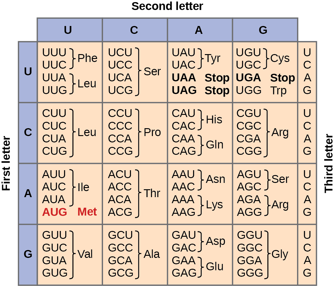
Figure 13.26 This photograph of Apollo 17 Commander Eugene Cernan driving the lunar rover on the Moon in 1972 looks as though it was taken at night with a large spotlight. In fact, the light is coming from the Sun. Because the acceleration due to gravity on the Moon is so low (about 1/6 that of Earth), the Moon’s escape velocity is much smaller. As a result, gas molecules escape very easily from the Moon, leaving it with virtually no atmosphere. Even during the daytime, the sky is black because there is no gas to scatter sunlight. (credit: Harrison H. Schmitt/NASA)

Paul Peter Urone and Roger Hinrichs, College Physics 2E, OpenStax. (credit: Harrison H. Schmitt/NASA) · CC BY-NC-SA 4.0 · Original image ↗ · Access for free ↗

Check Your Understanding

If you consider a very small object such as a grain of pollen, in a gas, then the number of and striking its surface would also be relatively small. Would the grain of pollen experience any fluctuations in pressure due to statistical fluctuations in the number of gas and striking it in a given amount of time?

Yes. Such fluctuations actually occur for a body of any size in a gas, but since the numbers of and are immense for macroscopic bodies, the fluctuations are a tiny percentage of the number of collisions, and the averages spoken of in this section vary imperceptibly. Roughly speaking the fluctuations are proportional to the inverse square root of the number of collisions, so for small bodies they can become significant. This was actually observed in the 19th century for pollen grains in water, and is known as the Brownian effect.

PhET Explorations

Gas Properties

Pump gas into a box and see what happens as you change the volume, add or remove heat, change gravity, and more. Measure the temperature and pressure, and discover how the properties of the gas vary in relation to each other.