Orbitals describe probability distributions; discrete energy differences produce discrete spectral transitions.
Quantum numbers and configurations
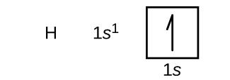
An orbital is specified by principal quantum number n = 1,2,…, angular momentum number ℓ = 0,…,n−1, and magnetic number mℓ = −ℓ,…,+ℓ. The s, p, d, and f subshells correspond to ℓ = 0,1,2,3 and hold 2,6,10,14 electrons. Each orbital holds at most two electrons with opposite spin by Pauli exclusion. Hund’s rule fills equivalent orbitals singly with parallel spin before pairing. Ground-state configurations usually follow increasing energy; hydrogen is 1s¹. For transition-metal cations, remove outer ns electrons before (n−1)d electrons.
An atom’s ground state is its lowest accessible electronic energy; excited states lie higher. Absorption requires photon energy matching an allowed upward transition, while downward transitions emit photons with hf = |ΔE|. The hydrogen Bohr model has En = −13.6 eV/n² and correctly captures its main energy-level spacing, though electron orbits are not literal modern quantum trajectories. Ionization raises an electron from a bound state to the continuum. An emission-line spectrum therefore reports discrete energy differences, whereas a continuous spectrum contains a broad range of energies.
Heisenberg uncertainty gives ΔxΔp ≥ ħ/2: arbitrarily exact simultaneous position and momentum are not available. In the photoelectric effect, emitted electrons have Kmax = hf − φ when photon energy exceeds the work function φ. Increasing intensity increases photon number at fixed frequency, not the energy of each photon; subthreshold light does not eject electrons in the elementary single-photon model. Species with unpaired electrons are paramagnetic and attracted to a field; species with all electrons paired are diamagnetic and weakly repelled.
Inner electrons partially shield outer electrons from nuclearcharge; effective nuclear charge Zeff is the attraction remaining after this shielding. Across a period, added protons generally increase Zeff experienced by valence electrons, drawing them inward. Down a group, occupied shells expand and shielding increases, usually increasing radius despite more protons. Within a shell, greater orbital penetration can lower an electron’s energy by allowing it to approach the nucleus. Treat Zeff as a useful model, not simply Z minus every other electron with equal weighting.
Try before revealing the answer. Hydrogen drops from n = 3 to n = 2. Find the emitted photon energy using En = −13.6 eV/n². Separately, is atomic nitrogen with 2p³ paramagnetic?
Worked answer
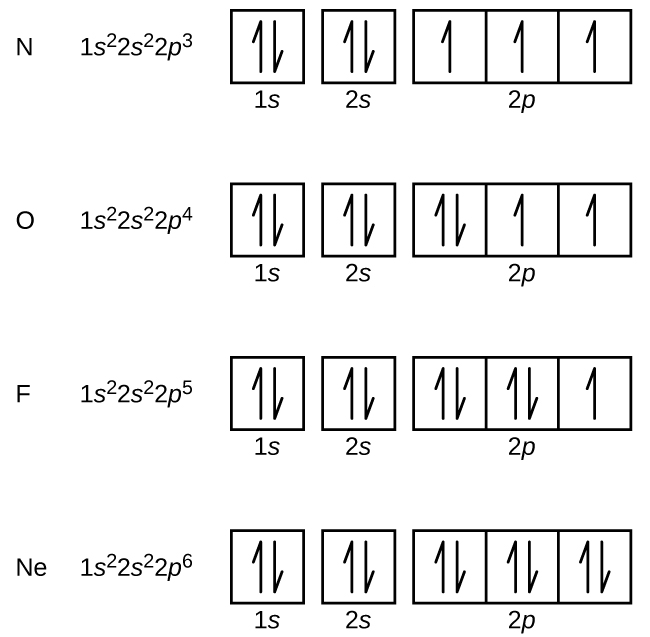
E₃ = −1.51 eV and E₂ = −3.40 eV, so the emitted photon has energy 1.89 eV. Nitrogen’s three 2p orbitals each contain one unpaired electron in the ground state, making the atom paramagnetic.
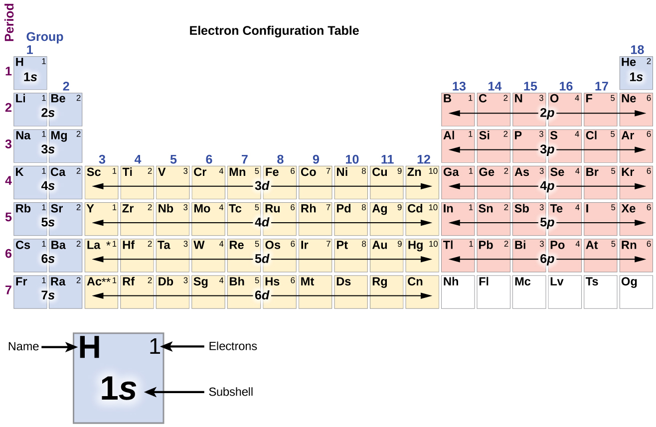
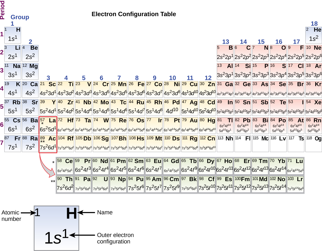
Figure 6.27 This partial periodic table shows electron configurations for the valence subshells of atoms. By “building up” from hydrogen, this table can be used to determine the electron configuration for atoms of most elements in the periodic table. (Electron configurations of the lanthanides and actinides are not accurately predicted by this simple approach. See Figure 6.29 .)
Figure 6.28 A core-abbreviated electron configuration (right) replaces the core electrons with the noble gas symbol whose configuration matches the core electron configuration of the other element.
Figure 6.29 This version of the periodic table shows the outer-shell electron configuration of each element. Note that down each group, the configuration is often similar.
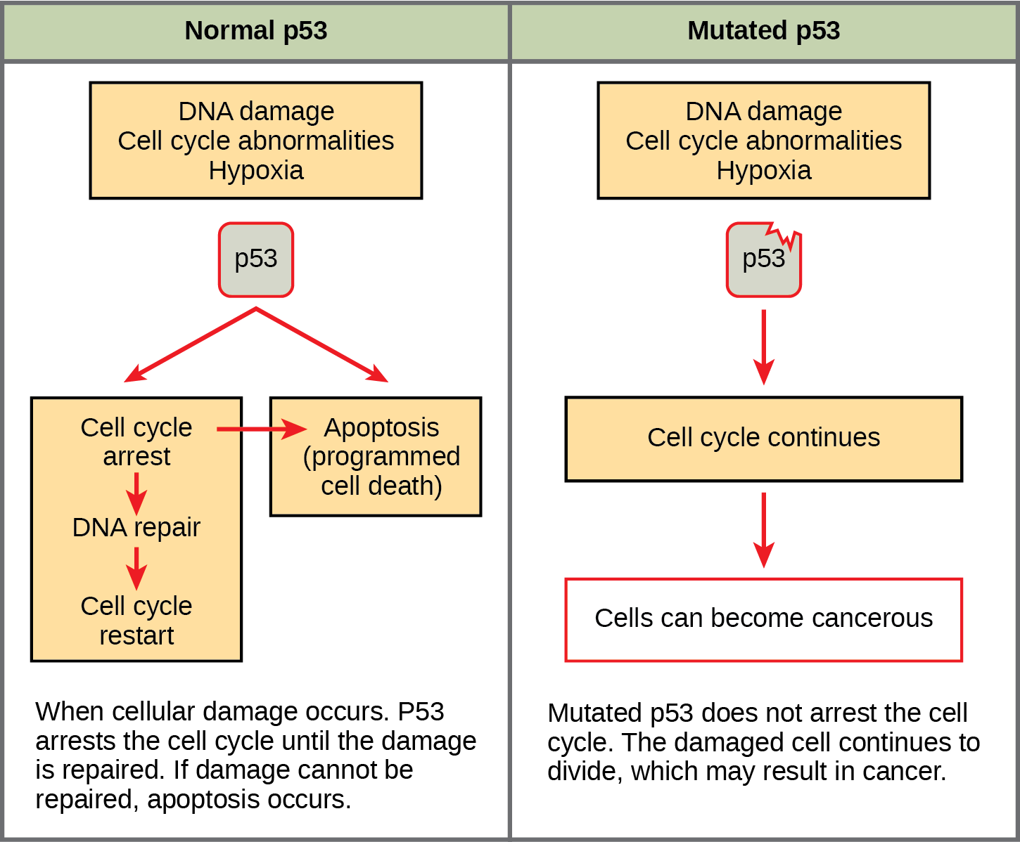
Figure 10.16 The role of normal p53 is to monitor DNA and the supply of oxygen (hypoxia is a condition of reduced oxygen supply). If damage is detected, p53 triggers repair mechanisms. If repairs are unsuccessful, p53 signals apoptosis. A cell with an abnormal p53 protein cannot repair damaged DNA and thus cannot signal apoptosis. Cells with abnormal p53 can become cancerous. (credit: modification of work by Thierry Soussi)
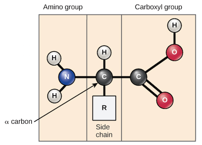
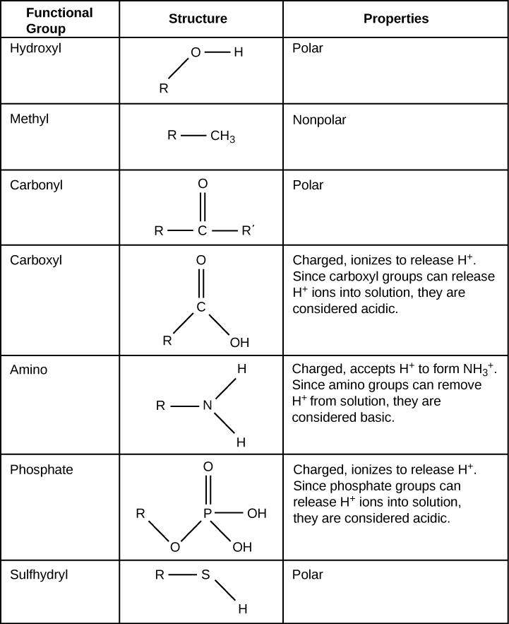
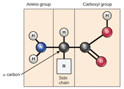
A nitrogen-containing functional group. A free amino acid’s amino group is typically protonated (NH₃⁺) near physiological pH; proline’s ring nitrogen is an exception to this formula.
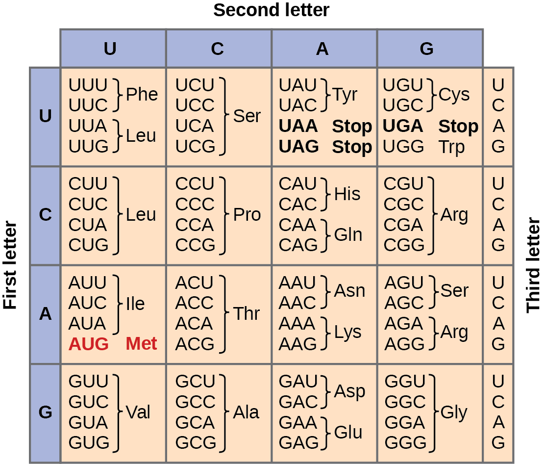
Figure 15.4 This figure shows the genetic code for translating each nucleotide triplet in mRNA into an amino acid or a termination signal in a protein. (credit: modification of work by NIH)
Figure 15.4 This figure shows the genetic code for translating each nucleotide triplet in mRNA into an amino acid or a termination signal in a protein. (credit: modification of work by NIH)
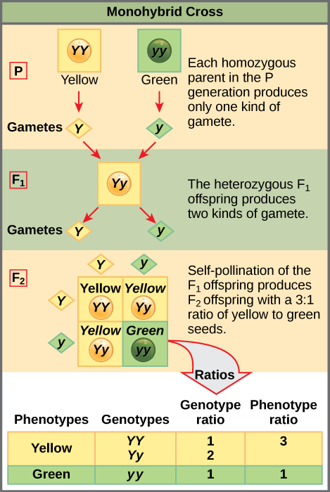
Figure 12.4 In the P generation, pea plants that are true-breeding for the dominant yellow phenotype are crossed with plants with the recessive green phenotype. This cross produces F 1 heterozygotes with a yellow phenotype. Punnett square analysis can be used to predict the genotypes of the F 2 generation.
An electrical property that can be positive or negative. Opposite charges attract and like charges repel; net charge is the sum of all charges on a particle.
Figure 15.4 This figure shows the genetic code for translating each nucleotide triplet in mRNA into an amino acid or a termination signal in a protein. (credit: modification of work by NIH)
Figure 12.4 In the P generation, pea plants that are true-breeding for the dominant yellow phenotype are crossed with plants with the recessive green phenotype. This cross produces F 1 heterozygotes with a yellow phenotype. Punnett square analysis can be used to predict the genotypes of the F 2 generation.
Figure 12.4 In the P generation, pea plants that are true-breeding for the dominant yellow phenotype are crossed with plants with the recessive green phenotype. This cross produces F 1 heterozygotes with a yellow phenotype. Punnett square analysis can be used to predict the genotypes of the F 2 generation.
The exponent needed to obtain a number from a chosen fixed number. For decimal logarithms, log₁₀(100) = 2 because 10² = 100; pH uses the negative decimal logarithm of hydrogen ion activity.
A thin boundary or sheet. Cell membranes are lipid bilayers containing proteins; blotting membranes are synthetic supports that hold proteins or nucleic acids for detection.
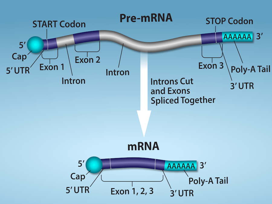
Figure 15.11 Eukaryotic pre-mRNA processing. In addition to 5’ Cap and 3’ Poly-A Tail addition, introns must be precisely removed and exons joined to generate a functional mRNA. Nucleotides upstream (towards the 5’cap) of the translation START codon are part of the 5’ untranslated region (5’ UTR). Nucleotides downstream (towards 3’end) of the STOP codon form the 3’ UTR. Both 5’ and 3’ UTRs are important for regulating translation initiation and mRNA stability. Credit: Rao, A., Ryan, K. Fletcher, S. and Tag, A. Department of Biology, Texas A&M University.
Rao, A., Ryan, K. Fletcher, S. and Tag, A. Department of Biology, Texas A&M University.; Mary Ann Clark, Matthew Douglas, and Jung Choi, Biology 2e, OpenStax. · CC BY-NC-SA 4.0
· Original image ↗ · Access for free ↗
Figure 12.4 In the P generation, pea plants that are true-breeding for the dominant yellow phenotype are crossed with plants with the recessive green phenotype. This cross produces F 1 heterozygotes with a yellow phenotype. Punnett square analysis can be used to predict the genotypes of the F 2 generation.
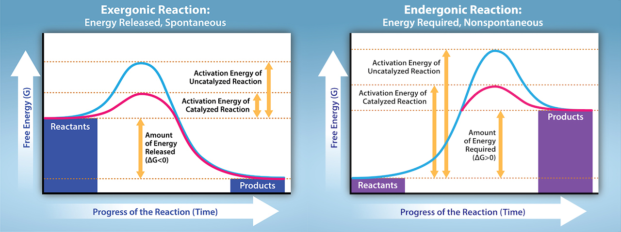
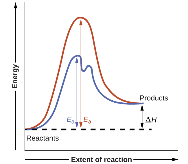
Figure 12.19 Reaction diagrams for an endothermic process in the absence (red curve) and presence (blue curve) of a catalyst. The catalyzed pathway involves a two-step mechanism (note the presence of two transition states) and an intermediate species (represented by the valley between the two transitions states).
Figure 15.4 This figure shows the genetic code for translating each nucleotide triplet in mRNA into an amino acid or a termination signal in a protein. (credit: modification of work by NIH)
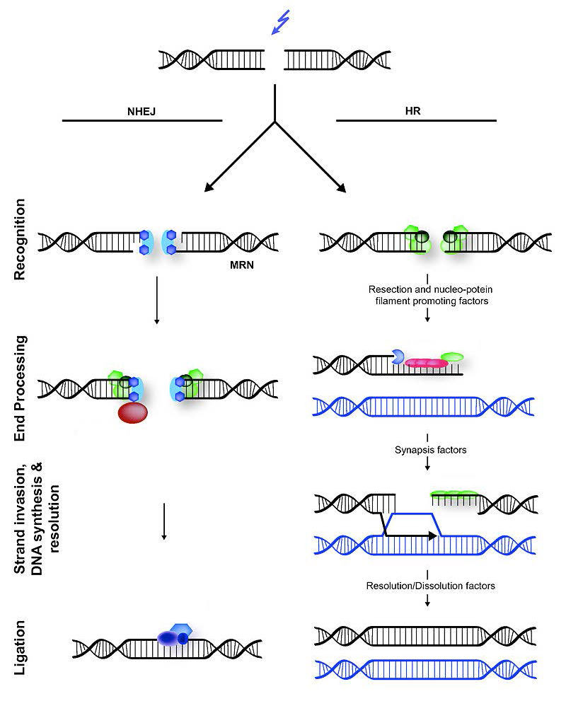
Figure 7.45 - Non-homologous end joining (left) versus homologous recombination (right) - Wikipedia
Wikipedia, as credited by Kevin Ahern, Indira Rajagopal, and Taralyn Tan, Biochemistry Free For All, Oregon State University, via Biology LibreTexts. · Source attribution
· Original image ↗ · Access for free ↗
The amount of a substance that can dissolve in a solvent under specified conditions. Soluble means able to dissolve; insoluble means only very slightly soluble in that solvent.
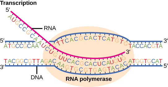
Figure 15.7 Messenger RNA is a copy of protein-coding information in the coding strand of DNA, with the substitution of U in the RNA for T in the coding sequence. However, new RNA nucleotides base pair with the nucleotides of the template strand. RNA is synthesized in its 5'-3' direction, using the enzyme RNA polymerase. As the template is read, the DNA unwinds ahead of the polymerase and then rewinds behind it.
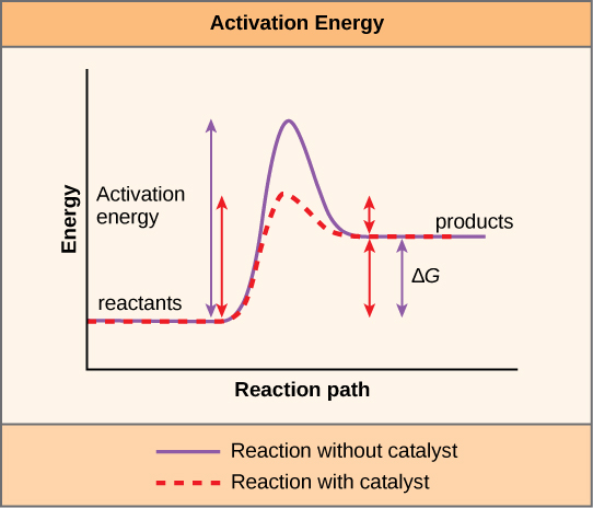
A fleeting, high-energy arrangement at a reaction barrier. It is an energy maximum along the reaction path, rather than a stable reaction intermediate.
Figure 12.19 Reaction diagrams for an endothermic process in the absence (red curve) and presence (blue curve) of a catalyst. The catalyzed pathway involves a two-step mechanism (note the presence of two transition states) and an intermediate species (represented by the valley between the two transitions states).
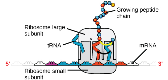
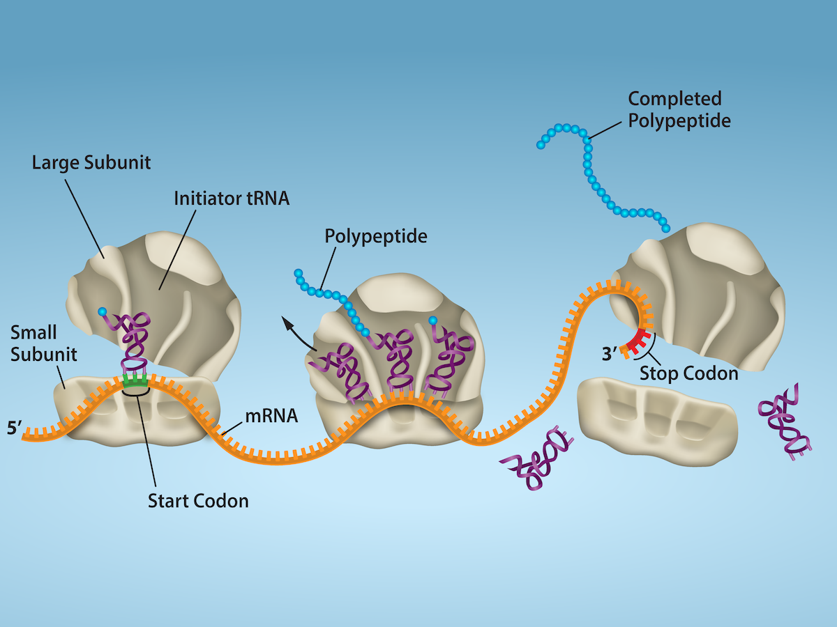
Figure 15.18 Translation begins when an initiator tRNA anticodon recognizes a start codon on mRNA bound to a small ribosomal subunit. The large ribosomal subunit joins the small subunit, and a second tRNA is recruited. As the mRNA moves relative to the ribosome, successive tRNAs move through the ribosome and the polypeptide chain is formed. Entry of a release factor into the A site terminates translation and the components dissociate.
No matching terms. Try a different name or abbreviation.
Chemistry 2E 6 — Summary
OpenStax · Chemistry 2E 6 — Summary ↗ Instructional page including learning objectives, examples, figures, source tables and questions. Site navigation and embedded media players are omitted; source media links remain available.
Light and other forms of electromagnetic radiation move through a vacuum with a constant speed, c, of 2.998 108 m s−1. This radiation shows wavelike behavior, which can be characterized by a frequency, ν, and a wavelength, λ, such that c = λν. Light is an example of a travelling wave. Other important wave phenomena include standing waves, periodic oscillations, and vibrations. Standing waves exhibit quantization, since their wavelengths are limited to discrete integer multiples of some characteristic lengths. Electromagnetic radiation that passes through two closely spaced narrow slits having dimensions roughly similar to the wavelength will show an interference pattern that is a result of constructive and destructive interference of the waves. Electromagnetic radiation also demonstrates properties of particles called photons. The energy of a photon is related to the frequency (or alternatively, the wavelength) of the radiation as E = hν (or ), where h is Planck's constant. That light demonstrates both wavelike and particle-like behavior is known as wave-particle duality. All forms of electromagnetic radiation share these properties, although various forms including X-rays, visible light, microwaves, and radio waves interact differently with matter and have very different practical applications. Electromagnetic radiation can be generated by exciting matter to higher energies, such as by heating it. The emitted light can be either continuous (incandescent sources like the sun) or discrete (from specific types of excited atoms). Continuous spectra often have distributions that can be approximated as blackbody radiation at some appropriate temperature. The line spectrum of hydrogen can be obtained by passing the light from an electrified tube of hydrogen gas through a prism. This line spectrum was simple enough that an empirical formula called the Rydberg formula could be derived from the spectrum. Three historically important paradoxes from the late 19th and early 20th centuries that could not be explained within the existing framework of classical mechanics and classical electromagnetism were the blackbody problem, the photoelectric effect, and the discrete spectra of atoms. The resolution of these paradoxes ultimately led to quantum theories that superseded the classical theories.
Bohr incorporated Planck’s and Einstein’s quantization ideas into a model of the hydrogen atom that resolved the paradox of atom stability and discrete spectra. The Bohr model of the hydrogen atom explains the connection between the quantization of photons and the quantized emission from atoms. Bohr described the hydrogen atom in terms of an electron moving in a circular orbit about a nucleus. He postulated that the electron was restricted to certain orbits characterized by discrete energies. Transitions between these allowed orbits result in the absorption or emission of photons. When an electron moves from a higher-energy orbit to a more stable one, energy is emitted in the form of a photon. To move an electron from a stable orbit to a more excited one, a photon of energy must be absorbed. Using the Bohr model, we can calculate the energy of an electron and the radius of its orbit in any one-electron system.
Macroscopic objects act as particles. Microscopic objects (such as electrons) have properties of both a particle and a wave. Their exact trajectories cannot be determined. The quantum mechanical model of atoms describes the three-dimensional position of the electron in a probabilistic manner according to a mathematical function called a wavefunction, often denoted as ψ. Atomic wavefunctions are also called orbitals. The squared magnitude of the wavefunction describes the distribution of the probability of finding the electron in a particular region in space. Therefore, atomic orbitals describe the areas in an atom where electrons are most likely to be found.
An atomic orbital is characterized by three quantum numbers. The principal quantum number, n, can be any positive integer. The general region for value of energy of the orbital and the average distance of an electron from the nucleus are related to n. Orbitals having the same value of n are said to be in the same shell. The secondary (angular momentum) quantum number, l, can have any integer value from 0 to n – 1. This quantum number describes the shape or type of the orbital. Orbitals with the same principal quantum number and the same l value belong to the same subshell. The magnetic quantum number, ml, with 2l + 1 values ranging from –l to +l, describes the orientation of the orbital in space. In addition, each electron has a spin quantum number, ms, that can be equal to No two electrons in the same atom can have the same set of values for all the four quantum numbers.
The relative energy of the subshells determine the order in which atomic orbitals are filled (1s, 2s, 2p, 3s, 3p, 4s, 3d, 4p, and so on). Electron configurations and orbital diagrams can be determined by applying the Pauli exclusion principle (no two electrons can have the same set of four quantum numbers) and Hund’s rule (whenever possible, electrons retain unpaired spins in degenerate orbitals).
Electrons in the outermost orbitals, called valence electrons, are responsible for most of the chemical behavior of elements. In the periodic table, elements with analogous valence electron configurations usually occur within the same group. There are some exceptions to the predicted filling order, particularly when half-filled or completely filled orbitals can be formed. The periodic table can be divided into three categories based on the orbital in which the last electron to be added is placed: main group elements (s and p orbitals), transition elements (d orbitals), and inner transition elements (f orbitals).
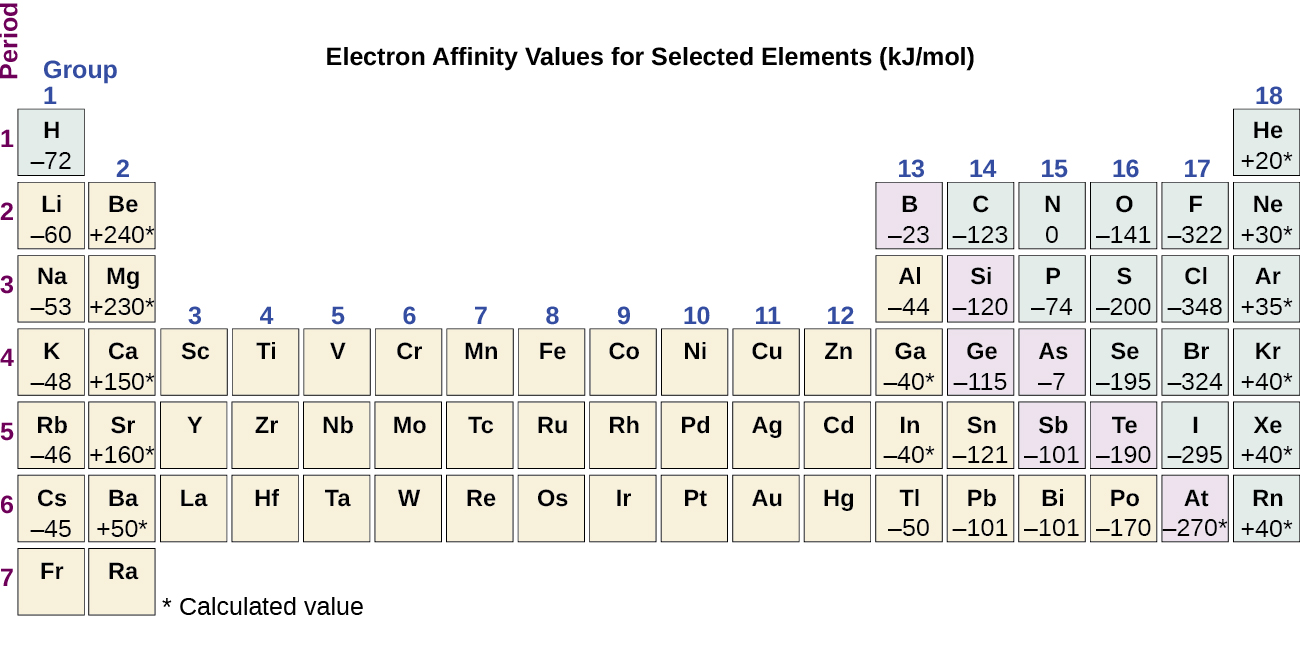
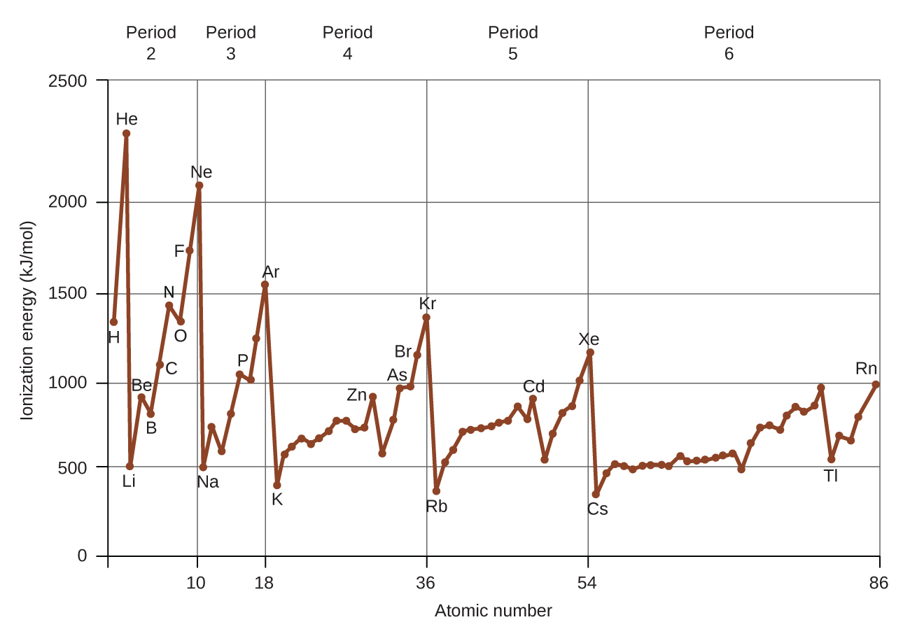
Electron configurations allow us to understand many periodic trends. Covalent radius increases as we move down a group because the n level (orbital size) increases. Covalent radius mostly decreases as we move left to right across a period because the effective nuclear charge experienced by the electrons increases, and the electrons are pulled in tighter to the nucleus. Anionic radii are larger than the parent atom, while cationic radii are smaller, because the number of valence electrons has changed while the nuclearcharge has remained constant. Ionization energy (the energy associated with forming a cation) decreases down a group and mostly increases across a period because it is easier to remove an electron from a larger, higher energy orbital. Electron affinity (the energy associated with forming an anion) is more favorable (exothermic) when electrons are placed into lower energy orbitals, closer to the nucleus. Therefore, electron affinity becomes increasingly negative as we move left to right across the periodic table and decreases as we move down a group. For both IE and electron affinity data, there are exceptions to the trends when dealing with completely filled or half-filled subshells.
6.4 Electronic Structure of Atoms (Electron Configurations)
Derive the predicted ground-state electron configurations of atoms
Identify and explain exceptions to predicted electron configurations for atoms and ions
Relate electron configurations to element classifications in the periodic table
Having introduced the basics of atomic structure and quantum mechanics, we can use our understanding of quantum numbers to determine how atomic orbitals relate to one another. This allows us to determine which orbitals are occupied by electrons in each atom. The specific arrangement of electrons in orbitals of an atom determines many of the chemical properties of that atom.
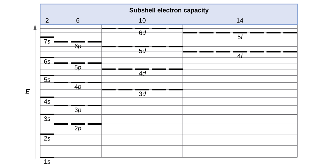
The energy of atomic orbitals increases as the principal quantum number, n, increases. In any atom with two or more electrons, the repulsion between the electrons makes energies of subshells with different values of l differ so that the energy of the orbitals increases within a shell in the order s < p < d < f.Figure 6.24 depicts how these two trends in increasing energy relate. The 1sorbital at the bottom of the diagram is the orbital with electrons of lowest energy. The energy increases as we move up to the 2s and then 2p, 3s, and 3p orbitals, showing that the increasing n value has more influence on energy than the increasing l value for small atoms. However, this pattern does not hold for larger atoms. The 3dorbital is higher in energy than the 4sorbital. Such overlaps continue to occur frequently as we move up the chart.
Figure 6.24 — 6.4 Electronic Structure of Atoms (Electron Configurations)
Figure 6.24 Generalized energy-level diagram for atomic orbitals in an atom with two or more electrons (not to scale).
Electrons in successive atoms on the periodic table tend to fill low-energy orbitals first. Thus, many students find it confusing that, for example, the 5p orbitals fill immediately after the 4d, and immediately before the 6s. The filling order is based on observed experimental results, and has been confirmed by theoretical calculations. As the principal quantum number, n, increases, the size of the orbital increases and the electrons spend more time farther from the nucleus. Thus, the attraction to the nucleus is weaker and the energy associated with the orbital is higher (less stabilized). But this is not the only effect we have to take into account. Within each shell, as the value of l increases, the electrons are less penetrating (meaning there is less electron density found close to the nucleus), in the order s > p > d > f. Electrons that are closer to the nucleus slightly repel electrons that are farther out, offsetting the more dominantelectron–nucleus attractions slightly (recall that all electrons have −1 charges, but nuclei have +Zcharges). This phenomenon is called shielding and will be discussed in more detail in the next section. Electrons in orbitals that experience more shielding are less stabilized and thus higher in energy. For small orbitals (1s through 3p), the increase in energy due to n is more significant than the increase due to l; however, for larger orbitals the two trends are comparable and cannot be simply predicted. We will discuss methods for remembering the observed order.
The letter that designates the orbital type (the subshell, l), and
A superscript number that designates the number of electrons in that particular subshell.
For example, the notation 2p4 (read "two–p–four") indicates four electrons in a p subshell (l = 1) with a principal quantum number (n) of 2. The notation 3d8 (read "three–d–eight") indicates eight electrons in the d subshell (i.e., l = 2) of the principal shell for which n = 3.
Figure 6.25 — 6.4 Electronic Structure of Atoms (Electron Configurations)
Figure 6.25 The diagram of an electron configuration specifies the subshell ( n and l value, with letter symbol) and superscript number of electrons.
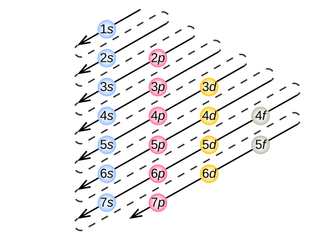
To determine the electronconfiguration for any particular atom, we can “build” the structures in the order of atomic numbers. Beginning with hydrogen, and continuing across the periods of the periodic table, we add one proton at a time to the nucleus and one electron to the proper subshell until we have described the electron configurations of all the elements. This procedure is called the Aufbau principle, from the German word Aufbau (“to build up”). Each added electron occupies the subshell of lowest energy available (in the order shown in Figure 6.24), subject to the limitations imposed by the allowed quantum numbers according to the Pauli exclusion principle. Electrons enter higher-energy subshells only after lower-energy subshells have been filled to capacity. Figure 6.26 illustrates the traditional way to remember the filling order for atomic orbitals. Since the arrangement of the periodic table is based on the electron configurations, Figure 6.27 provides an alternative method for determining the electronconfiguration. The filling order simply begins at hydrogen and includes each subshell as you proceed in increasing Z order. For example, after filling the 3p block up to Ar, we see the orbital will be 4s (K, Ca), followed by the 3d orbitals.
Figure 6.26 — 6.4 Electronic Structure of Atoms (Electron Configurations)
Figure 6.26 This diagram depicts the energy order for atomic orbitals and is useful for deriving ground-state electron configurations.
Figure 6.27 — 6.4 Electronic Structure of Atoms (Electron Configurations)
Figure 6.27 This partial periodic table shows electron configurations for the valence subshells of atoms. By “building up” from hydrogen, this table can be used to determine the electron configuration for atoms of most elements in the periodic table. (Electron configurations of the lanthanides and actinides are not accurately predicted by this simple approach. See Figure 6.29 .)
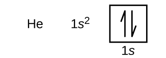
Following hydrogen is the noble gas helium, which has an atomic number of 2. The helium atom contains two protons and two electrons. The first electron has the same four quantum numbers as the hydrogen atomelectron (n = 1, l = 0, ml = 0, ). The second electron also goes into the 1sorbital and fills that orbital. The second electron has the same n, l, and ml quantum numbers, but must have the opposite spin quantum number, This is in accord with the Pauli exclusion principle: No two electrons in the same atom can have the same set of four quantum numbers. For orbital diagrams, this means two arrows go in each box (representing two electrons in each orbital) and the arrows must point in opposite directions (representing paired spins). The electronconfiguration and orbital diagram of helium are:
The n = 1 shell is completely filled in a helium atom.
An atom of boron (atomic number 5) contains five electrons. The n = 1 shell is filled with two electrons and three electrons will occupy the n = 2 shell. Because any s subshell can contain only two electrons, the fifth electron must occupy the next energy level, which will be a 2porbital. There are three degenerate 2p orbitals (ml = −1, 0, +1) and the electron can occupy any one of these p orbitals. When drawing orbital diagrams, we include empty boxes to depict any empty orbitals in the same subshell that we are filling.
Carbon (atomic number 6) has six electrons. Four of them fill the 1s and 2s orbitals. The remaining two electrons occupy the 2p subshell. We now have a choice of filling one of the 2p orbitals and pairing the electrons or of leaving the electrons unpaired in two different, but degenerate, p orbitals. The orbitals are filled as described by Hund’s rule: the lowest-energy configuration for an atom with electrons within a set of degenerate orbitals is that having the maximum number of unpaired electrons. Thus, the two electrons in the carbon 2p orbitals have identical n, l, and ms quantum numbers and differ in their ml quantum number (in accord with the Pauli exclusion principle). The electronconfiguration and orbital diagram for carbon are:
Nitrogen (atomic number 7) fills the 1s and 2s subshells and has one electron in each of the three 2p orbitals, in accordance with Hund’s rule. These three electrons have unpaired spins. Oxygen (atomic number 8) has a pair of electrons in any one of the 2p orbitals (the electrons have opposite spins) and a single electron in each of the other two. Fluorine (atomic number 9) has only one 2porbital containing an unpaired electron. All of the electrons in the noble gas neon (atomic number 10) are paired, and all of the orbitals in the n = 1 and the n = 2 shells are filled. The electron configurations and orbital diagrams of these four elements are:
The alkali metal sodium (atomic number 11) has one more electron than the neon atom. This electron must go into the lowest-energy subshell available, the 3sorbital, giving a 1s22s22p63s1configuration. The electrons occupying the outermost shell orbital(s) (highest value of n) are called valence electrons, and those occupying the inner shell orbitals are called core electrons (Figure 6.28). Since the core electron shells correspond to noble gas electron configurations, we can abbreviate electron configurations by writing the noble gas that matches the core electronconfiguration, along with the valence electrons in a condensed format. For our sodium example, the symbol [Ne] represents core electrons, (1s22s22p6) and our abbreviated or condensed configuration is [Ne]3s1.
Figure 6.28 — 6.4 Electronic Structure of Atoms (Electron Configurations)
Figure 6.28 A core-abbreviated electron configuration (right) replaces the core electrons with the noble gas symbol whose configuration matches the core electron configuration of the other element.
Similarly, the abbreviated configuration of lithium can be represented as [He]2s1, where [He] represents the configuration of the helium atom, which is identical to that of the filled inner shell of lithium. Writing the configurations in this way emphasizes the similarity of the configurations of lithium and sodium. Both atoms, which are in the alkali metal family, have only one electron in a valence s subshell outside a filled set of inner shells.
The alkaline earth metal magnesium (atomic number 12), with its 12 electrons in a [Ne]3s2configuration, is analogous to its family member beryllium, [He]2s2. Both atoms have a filled s subshell outside their filled inner shells. Aluminum (atomic number 13), with 13 electrons and the electronconfiguration [Ne]3s23p1, is analogous to its family member boron, [He]2s22p1.
The electron configurations of silicon (14 electrons), phosphorus (15 electrons), sulfur (16 electrons), chlorine (17 electrons), and argon (18 electrons) are analogous in the electron configurations of their outer shells to their corresponding family members carbon, nitrogen, oxygen, fluorine, and neon, respectively, except that the principal quantum number of the outer shell of the heavier elements has increased by one to n = 3. Figure 6.29 shows the lowest energy, or ground-state, electronconfiguration for these elements as well as that for atoms of each of the known elements.
Figure 6.29 — 6.4 Electronic Structure of Atoms (Electron Configurations)
Figure 6.29 This version of the periodic table shows the outer-shell electron configuration of each element. Note that down each group, the configuration is often similar.
When we come to the next element in the periodic table, the alkali metal potassium (atomic number 19), we might expect that we would begin to add electrons to the 3d subshell. However, all available chemical and physical evidence indicates that potassium is like lithium and sodium, and that the next electron is not added to the 3d level but is, instead, added to the 4s level (Figure 6.29). As discussed previously, the 3dorbital with no radial nodes is higher in energy because it is less penetrating and more shielded from the nucleus than the 4s, which has three radial nodes. Thus, potassium has an electronconfiguration of [Ar]4s1. Hence, potassium corresponds to Li and Na in its valence shell configuration. The next electron is added to complete the 4s subshell and calcium has an electronconfiguration of [Ar]4s2. This gives calcium an outer-shell electronconfiguration corresponding to that of beryllium and magnesium.
Beginning with the transition metal scandium (atomic number 21), additional electrons are added successively to the 3d subshell. This subshell is filled to its capacity with 10 electrons (remember that for l = 2 [d orbitals], there are 2l + 1 = 5 values of ml, meaning that there are five d orbitals that have a combined capacity of 10 electrons). The 4p subshell fills next. Note that for three series of elements, scandium (Sc) through copper (Cu), yttrium (Y) through silver (Ag), and lanthanum (La) through gold (Au), a total of 10 delectrons are successively added to the (n – 1) shell next to the n shell to bring that (n – 1) shell from 8 to 18 electrons. For two series, lanthanum (La) through lutetium (Lu) and actinium (Ac) through lawrencium (Lr), 14 felectrons (l = 3, 2l + 1 = 7 ml values; thus, seven orbitals with a combined capacity of 14 electrons) are successively added to the (n – 2) shell to bring that shell from 18 electrons to a total of 32 electrons.
The atomic number of phosphorus is 15. Thus, a phosphorus atom contains 15 electrons. The order of filling of the energy levels is 1s, 2s, 2p, 3s, 3p, 4s, . . . The 15 electrons of the phosphorus atom will fill up to the 3porbital, which will contain three electrons:
The last electron added is a 3pelectron. Therefore, n = 3 and, for a p-type orbital, l = 1. The ml value could be –1, 0, or +1. The three p orbitals are degenerate, so any of these ml values is correct. For unpaired electrons, convention assigns the value of for the spin quantum number; thus,
Check Your Learning
Identify the atoms from the electron configurations given:
(a) [Ar]4s23d5
(b) [Kr]5s24d105p6
Answer:
(a) Mn (b) Xe
The periodic table can be a powerful tool in predicting the electronconfiguration of an element. However, we do find exceptions to the order of filling of orbitals that are shown in Figure 6.26 or Figure 6.27. For instance, the electron configurations (shown in Figure 6.29) of the transition metals chromium (Cr; atomic number 24) and copper (Cu; atomic number 29), among others, are not those we would expect. In general, such exceptions involve subshells with very similar energy, and small effects can lead to changes in the order of filling.
In the case of Cr and Cu, we find that half-filled and completely filled subshells apparently represent conditions of preferred stability. This stability is such that an electron shifts from the 4s into the 3dorbital to gain the extra stability of a half-filled 3d subshell (in Cr) or a filled 3d subshell (in Cu). Other exceptions also occur. For example, niobium (Nb, atomic number 41) is predicted to have the electronconfiguration [Kr]5s24d3. Experimentally, we observe that its ground-state electronconfiguration is actually [Kr]5s14d4. We can rationalize this observation by saying that the electron–electron repulsions experienced by pairing the electrons in the 5sorbital are larger than the gap in energy between the 5s and 4d orbitals. There is no simple method to predict the exceptions for atoms where the magnitude of the repulsions between electrons is greater than the small differences in energy between subshells.
As described earlier, the periodic table arranges atoms based on increasing atomic number so that elements with the same chemical properties recur periodically. When their electron configurations are added to the table (Figure 6.29), we also see a periodic recurrence of similar electron configurations in the outer shells of these elements. Because they are in the outer shells of an atom, valence electrons play the most important role in chemical reactions. The outer electrons have the highest energy of the electrons in an atom and are more easily lost or shared than the core electrons. Valence electrons are also the determining factor in some physical properties of the elements.
Elements in any one group (or column) have the same number of valence electrons; the alkali metals lithium and sodium each have only one valence electron, the alkaline earth metals beryllium and magnesium each have two, and the halogens fluorine and chlorine each have seven valence electrons. The similarity in chemical properties among elements of the same group occurs because they have the same number of valence electrons. It is the loss, gain, or sharing of valence electrons that defines how elements react.
It is important to remember that the periodic table was developed on the basis of the chemical behavior of the elements, well before any idea of their atomic structure was available. Now we can understand why the periodic table has the arrangement it has—the arrangement puts elements whose atoms have the same number of valence electrons in the same group. This arrangement is emphasized in Figure 6.29, which shows in periodic-table form the electronconfiguration of the last subshell to be filled by the Aufbau principle. The colored sections of Figure 6.29 show the three categories of elements classified by the orbitals being filled: main group, transition, and inner transition elements. These classifications determine which orbitals are counted in the valence shell, or highest energy level orbitals of an atom.
Main group elements (sometimes called representative elements) are those in which the last electron added enters an s or a porbital in the outermost shell, shown in blue and red in Figure 6.29. This category includes all the nonmetallic elements, as well as many metals and the metalloids. The valence electrons for main group elements are those with the highest n level. For example, gallium (Ga, atomic number 31) has the electronconfiguration [Ar]4s23d104p1, which contains three valence electrons (underlined). The completely filled d orbitals count as core, not valence, electrons.
Transition elements or transition metals. These are metallic elements in which the last electron added enters a dorbital. The valence electrons (those added after the last noble gas configuration) in these elements include the ns and (n – 1) delectrons. The official IUPAC definition of transition elements specifies those with partially filled d orbitals. Thus, the elements with completely filled orbitals (Zn, Cd, Hg, as well as Cu, Ag, and Au in Figure 6.29) are not technically transition elements. However, the term is frequently used to refer to the entire d block (colored yellow in Figure 6.29), and we will adopt this usage in this textbook.
Inner transition elements are metallic elements in which the last electron added occupies an forbital. They are shown in green in Figure 6.29. The valence shells of the inner transition elements consist of the (n – 2)f, the (n – 1)d, and the ns subshells. There are two inner transition series:
The lanthanide series: lanthanum (La) through lutetium (Lu)
The actinide series: actinium (Ac) through lawrencium (Lr)
Lanthanum and actinium, because of their similarities to the other members of the series, are included and used to name the series, even though they are transition metals with no felectrons.
Ions are formed when atoms gain or lose electrons. A cation (positively chargedion) forms when one or more electrons are removed from a parent atom. For main group elements, the electrons that were added last are the first electrons removed. For transition metals and inner transition metals, however, electrons in the sorbital are easier to remove than the d or felectrons, and so the highest nselectrons are lost, and then the (n – 1)d or (n – 2)felectrons are removed. An anion (negatively chargedion) forms when one or more electrons are added to a parent atom. The added electrons fill in the order predicted by the Aufbau principle.
First, write out the electronconfiguration for each parent atom. We have chosen to show the full, unabbreviated configurations to provide more practice for students who want it, but listing the core-abbreviated electron configurations is also acceptable.
(d) Fe: 1s22s22p63s23p64s23d6. Iron(II) loses two electrons and, since it is a transition metal, they are removed from the 4sorbital Fe2+: 1s22s22p63s23p64s23d6 = 1s22s22p63s23p63d6.
(e). Sm: 1s22s22p63s23p64s23d104p65s24d105p66s24f6. Samarium trication loses three electrons. The first two will be lost from the 6sorbital, and the final one is removed from the 4forbital. Sm3+: 1s22s22p63s23p64s23d104p65s24d105p66s24f6 = 1s22s22p63s23p64s23d104p65s24d105p64f5.