Use a model to predict a perturbation, then identify evidence that could separate competing explanations.
Perturb one variable within a stated model
Translate a proposed intervention into the variable it changes. In a simple independent binding model, fractional occupancy is L/(Kd+L); increasing ligand raises occupancy toward a ceiling. A prediction assumes constant receptor number, unchanged affinity, and an appropriate equilibrium measurement. If an intervention changes several variables, derive conditional predictions rather than presenting one as inevitable. Test extreme cases: zero ligand gives zero occupancy, while very high ligand approaches complete occupancy. These limits often expose a mistaken reciprocal or sign.
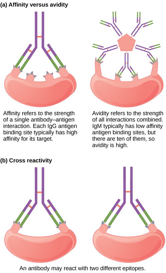
A reduced cellular response could reflect fewer receptors, weaker binding, or impaired downstream signaling. Measure abundance, binding, and signaling separately; a single output cannot distinguish all three. A rescue experiment can support a pathway but may have off-target effects. Prefer a comparison for which the competing models predict different outcomes, using matched controls. Evidence that both models predict can be consistent with each but does little to choose between them. Failure to reject one explanation is not proof that it is uniquely correct.
Write the relation before substituting numbers, cancel units, and predict whether the answer should increase or decrease. A rate proportional to r⁴ increases sixteenfold if r doubles, provided other variables stay fixed. A 20% decrease followed by a 20% increase yields 0.8×1.2 = 0.96 of the start, not complete recovery. Approximate powers of ten before exact arithmetic. If the result contradicts a limiting case or violates a physical bound, revisit the model, unit conversion, and algebra before selecting it.
Question. At L = Kd occupancy is 1/2. A drug halves Kd while leaving free L fixed at its original value. What is the new occupancy? If maximum response falls instead, does this alone prove receptoraffinity decreased?
Show reasoning
New occupancy is L/(L/2+L) = 2/3. Increased affinity raises occupancy at the chosen concentration but does not guarantee a proportionate functional response. A lower maximum response could involve receptor abundance or downstream capacity; saturation binding and signaling controls are needed. The observation alone does not establish lower affinity.
Figure 2.7 Seeing a police car behind you would probably affect your driving behavior. (credit: Michael Gil)
Rose M. Spielman, William J. Jenkins, and Marilyn D. Lovett, Psychology 2E, OpenStax. (credit: Michael Gil) · CC BY-NC-SA 4.0
· Original image ↗ · Access for free ↗Figure 2.8 — 2.2 Approaches to Research
Figure 2.8 (a) Jane Goodall made a career of conducting naturalistic observations of (b) chimpanzee behavior. (credit “Jane Goodall”: modification of work by Erik Hersman; “chimpanzee”: modification of work by “Afrika Force”/Flickr.com)
Rose M. Spielman, William J. Jenkins, and Marilyn D. Lovett, Psychology 2E, OpenStax. (credit “Jane Goodall”: modification of work by Erik Hersman; “chimpanzee”: modification of work by “Afrika Force”/Flickr.com) · CC BY-NC-SA 4.0
· Original image ↗ · Access for free ↗Figure 2.9 — 2.2 Approaches to Research
Figure 2.9 Surveys can be administered in a number of ways, including electronically administered research, like the survey shown here. (credit: Robert Nyman)
Rose M. Spielman, William J. Jenkins, and Marilyn D. Lovett, Psychology 2E, OpenStax. (credit: Robert Nyman) · CC BY-NC-SA 4.0
· Original image ↗ · Access for free ↗Figure 2.10 — 2.2 Approaches to Research
Figure 2.10 A researcher doing archival research examines records, whether archived as a (a) hardcopy or (b) electronically. (credit “paper files”: modification of work by “Newtown graffiti”/Flickr; “computer”: modification of work by INPIVIC Family/Flickr)
Rose M. Spielman, William J. Jenkins, and Marilyn D. Lovett, Psychology 2E, OpenStax. (credit “paper files”: modification of work by “Newtown graffiti”/Flickr; “computer”: modification of work by INPIVIC Family/Flickr) · CC BY-NC-SA 4.0
· Original image ↗ · Access for free ↗Figure 2.11 — 2.2 Approaches to Research
Figure 2.11 Longitudinal research like the CPS-3 help us to better understand how smoking is associated with cancer and other diseases. (credit: CDC/Debora Cartagena)
Figure 4.26 - A Lineweaver-Burk plot of 1/V₀ vs 1/[S]. Image by Aleia Kim
Kevin Ahern, Indira Rajagopal, and Taralyn Tan, Biochemistry Free For All, Oregon State University, via Biology LibreTexts. Image by Aleia Kim · CC BY-NC-SA 4.0
· Original image ↗ · Access for free ↗
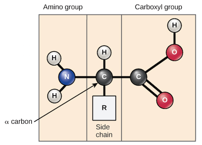
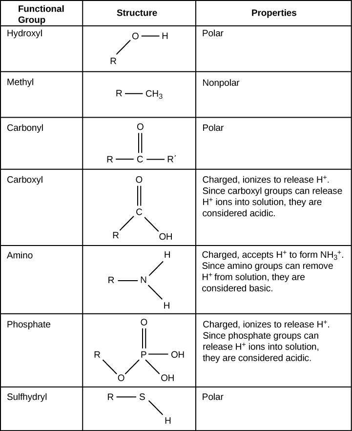
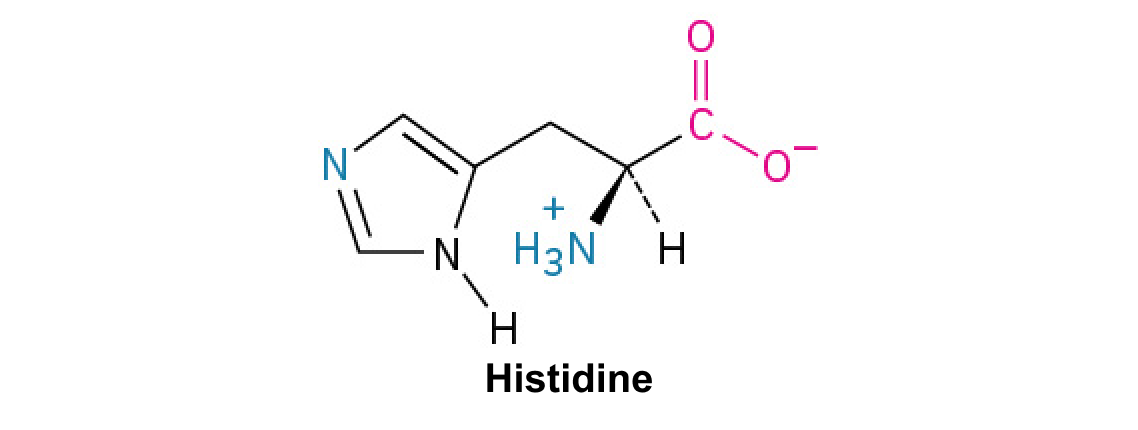
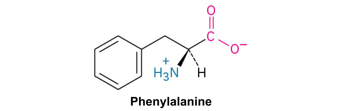
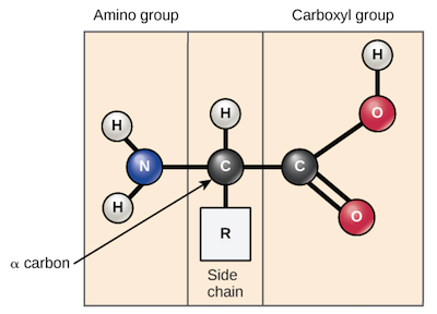
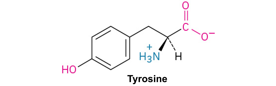
A nitrogen-containing functional group. A free amino acid’s amino group is typically protonated (NH₃⁺) near physiological pH; proline’s ring nitrogen is an exception to this formula.
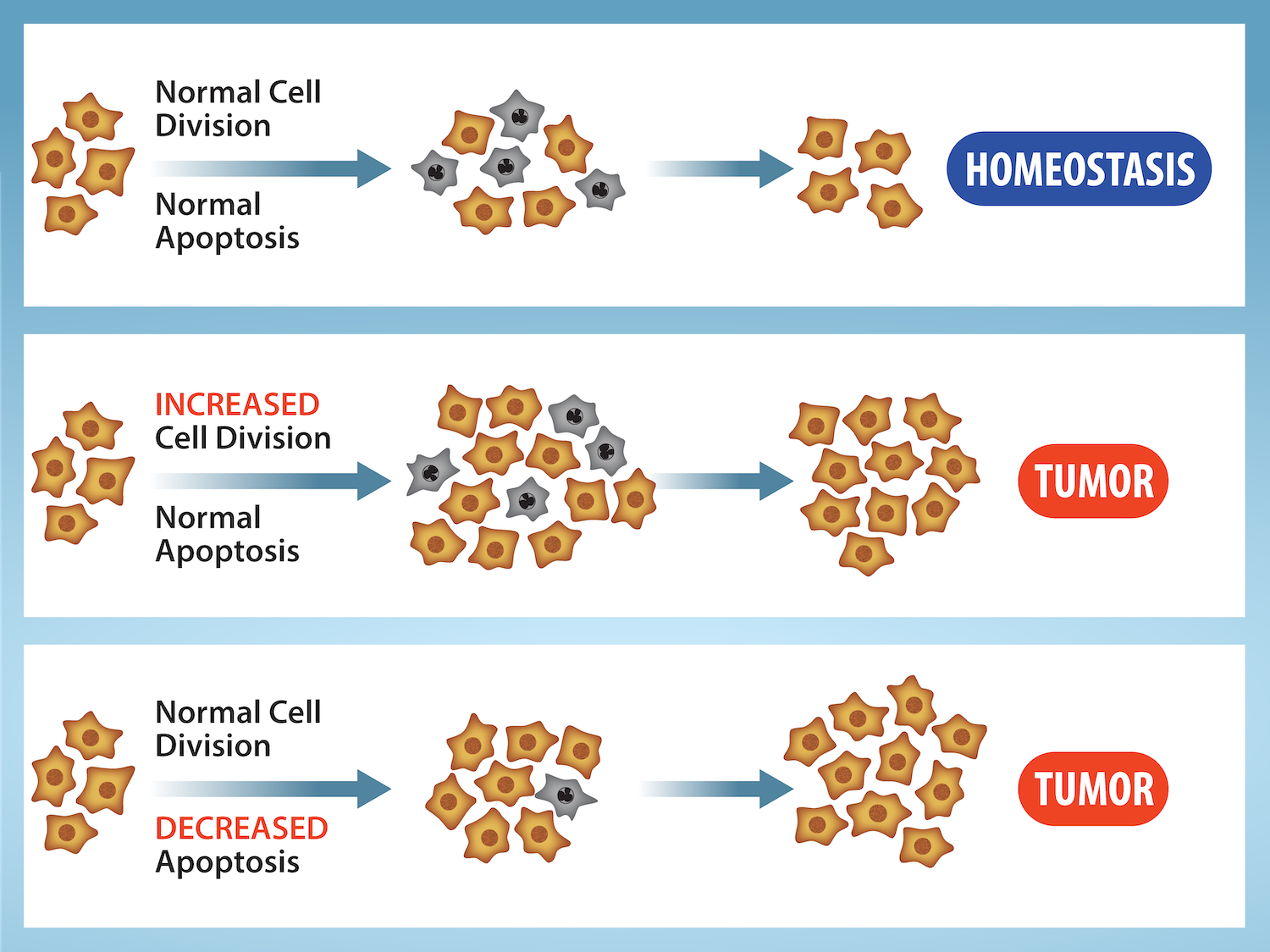
Figure 10.15 Cell Division and Apoptosis. In an adult organism, normal cell division is balanced by apoptosis (programmed cell death) to maintain a constant cell number in homeostasis. Either an increase in cell division or a decrease in apoptosis leads an increase in the number of cells and tumor formation. Credit: Rao, A. and Ryan, K. Department of Biology, Texas A&M University.
Rao, A. and Ryan, K. Department of Biology, Texas A&M University. Mary Ann Clark, Matthew Douglas, and Jung Choi, Biology 2e, OpenStax. · CC BY-NC-SA 4.0
· Original image ↗ · Access for free ↗
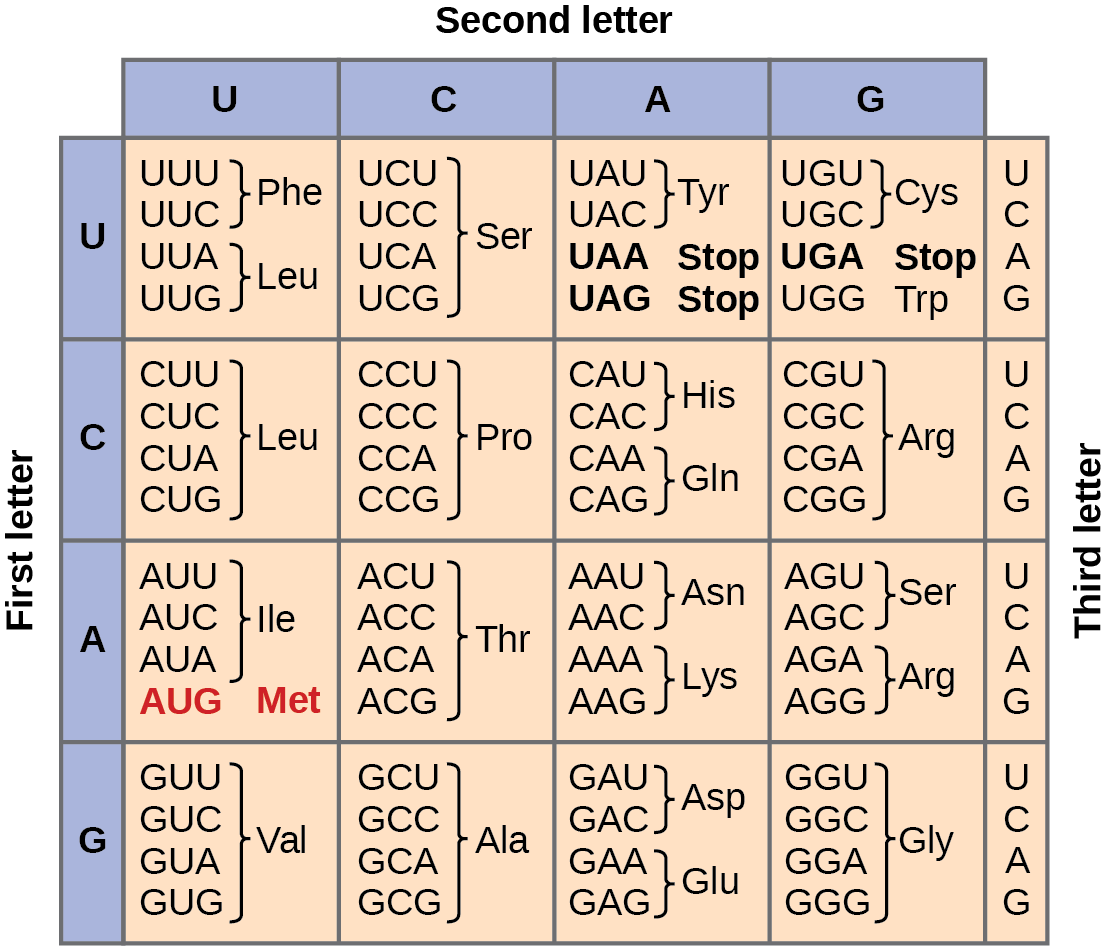
Figure 15.4 This figure shows the genetic code for translating each nucleotide triplet in mRNA into an amino acid or a termination signal in a protein. (credit: modification of work by NIH)
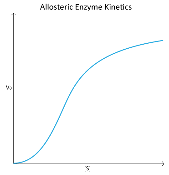
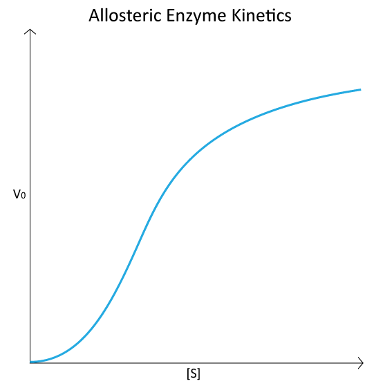
Figure 4.44 - Kinetic profile of an allosteric enzyme whose activity is controlled by a homotropic effector. Image by Aleia Kim
Kevin Ahern, Indira Rajagopal, and Taralyn Tan, Biochemistry Free For All, Oregon State University, via Biology LibreTexts. Image by Aleia Kim · CC BY-NC-SA 4.0
· Original image ↗ · Access for free ↗
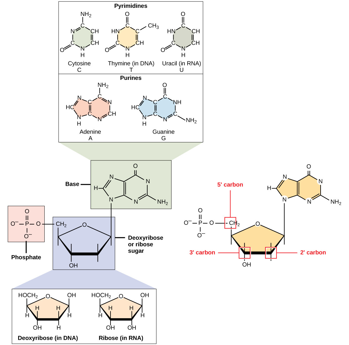
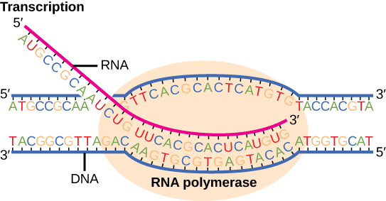
Figure 15.7 Messenger RNA is a copy of protein-coding information in the coding strand of DNA, with the substitution of U in the RNA for T in the coding sequence. However, new RNA nucleotides base pair with the nucleotides of the template strand. RNA is synthesized in its 5'-3' direction, using the enzyme RNA polymerase. As the template is read, the DNA unwinds ahead of the polymerase and then rewinds behind it.
An electrical property that can be positive or negative. Opposite charges attract and like charges repel; net charge is the sum of all charges on a particle.
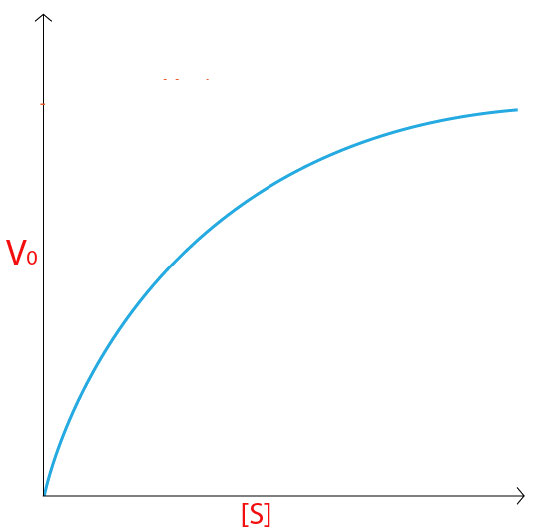
Figure 4.18 - Kinetics of an enzyme obeying Michaelis-Menten kinetics. Image by Aleia Kim
Kevin Ahern, Indira Rajagopal, and Taralyn Tan, Biochemistry Free For All, Oregon State University, via Biology LibreTexts. Image by Aleia Kim · CC BY-NC-SA 4.0
· Original image ↗ · Access for free ↗
A ratio of product to reactant activities at equilibrium, each raised to its stoichiometric coefficient. At a fixed temperature, a catalyst does not change this ratio.
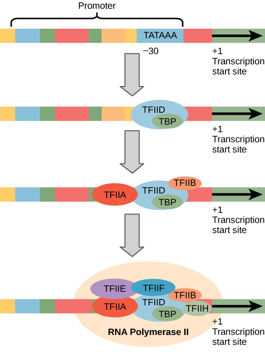
Figure 15.10 A generalized promoter of a gene transcribed by RNA polymerase II is shown. Transcription factors recognize the promoter. RNA polymerase II then binds and forms the transcription initiation complex.
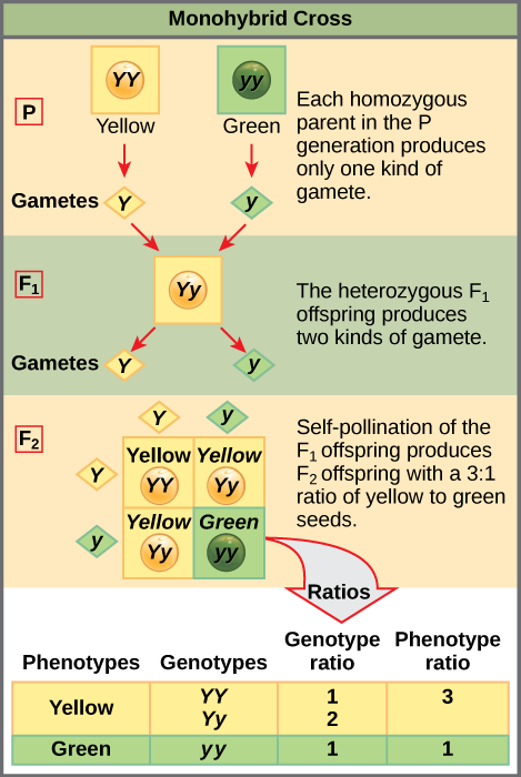
Figure 12.4 In the P generation, pea plants that are true-breeding for the dominant yellow phenotype are crossed with plants with the recessive green phenotype. This cross produces F 1 heterozygotes with a yellow phenotype. Punnett square analysis can be used to predict the genotypes of the F 2 generation.
Figure 4.18 - Kinetics of an enzyme obeying Michaelis-Menten kinetics. Image by Aleia Kim
Kevin Ahern, Indira Rajagopal, and Taralyn Tan, Biochemistry Free For All, Oregon State University, via Biology LibreTexts. Image by Aleia Kim · CC BY-NC-SA 4.0
· Original image ↗ · Access for free ↗
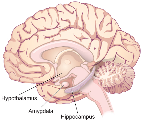
hypothalamus
Forebrain region coordinating homeostatic, endocrine, and autonomic functions.
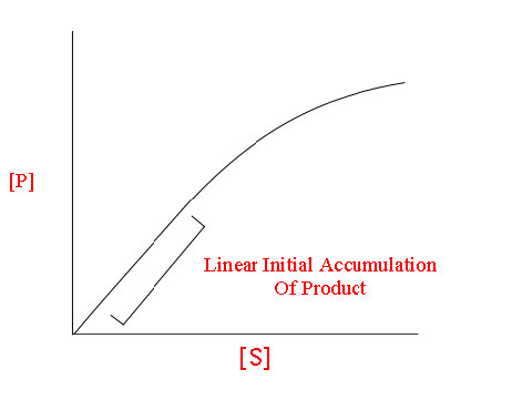
The early rate of product formation, measured before substantial substrate depletion or product accumulation, usually after the brief binding transient.
Figure 4.18 - Kinetics of an enzyme obeying Michaelis-Menten kinetics. Image by Aleia Kim
Kevin Ahern, Indira Rajagopal, and Taralyn Tan, Biochemistry Free For All, Oregon State University, via Biology LibreTexts. Image by Aleia Kim · CC BY-NC-SA 4.0
· Original image ↗ · Access for free ↗
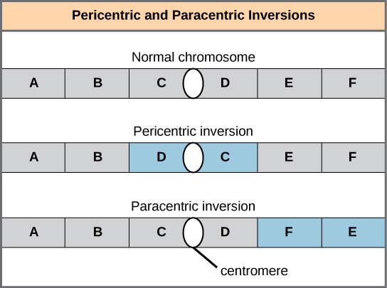
Figure 13.11 Pericentric inversions include the centromere, and paracentric inversions do not. A pericentric inversion can change the chromosome arms' relative lengths. A paracentric inversion cannot.
Figure 4.26 - A Lineweaver-Burk plot of 1/V₀ vs 1/[S]. Image by Aleia Kim
Kevin Ahern, Indira Rajagopal, and Taralyn Tan, Biochemistry Free For All, Oregon State University, via Biology LibreTexts. Image by Aleia Kim · CC BY-NC-SA 4.0
· Original image ↗ · Access for free ↗
The exponent needed to obtain a number from a chosen fixed number. For decimal logarithms, log₁₀(100) = 2 because 10² = 100; pH uses the negative decimal logarithm of hydrogen ion activity.
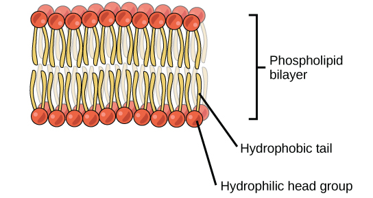
A thin boundary or sheet. Cell membranes are lipid bilayers containing proteins; blotting membranes are synthetic supports that hold proteins or nucleic acids for detection.
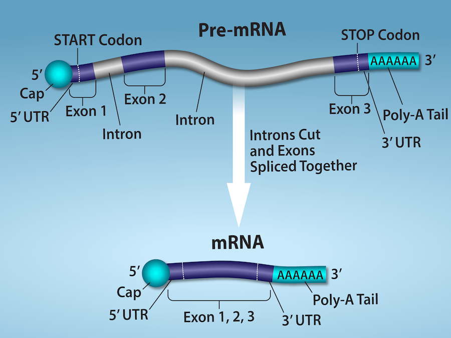
Figure 15.11 Eukaryotic pre-mRNA processing. In addition to 5’ Cap and 3’ Poly-A Tail addition, introns must be precisely removed and exons joined to generate a functional mRNA. Nucleotides upstream (towards the 5’cap) of the translation START codon are part of the 5’ untranslated region (5’ UTR). Nucleotides downstream (towards 3’end) of the STOP codon form the 3’ UTR. Both 5’ and 3’ UTRs are important for regulating translation initiation and mRNA stability. Credit: Rao, A., Ryan, K. Fletcher, S. and Tag, A. Department of Biology, Texas A&M University.
Rao, A., Ryan, K. Fletcher, S. and Tag, A. Department of Biology, Texas A&M University.; Mary Ann Clark, Matthew Douglas, and Jung Choi, Biology 2e, OpenStax. · CC BY-NC-SA 4.0
· Original image ↗ · Access for free ↗
Figure 4.18 - Kinetics of an enzyme obeying Michaelis-Menten kinetics. Image by Aleia Kim
Kevin Ahern, Indira Rajagopal, and Taralyn Tan, Biochemistry Free For All, Oregon State University, via Biology LibreTexts. Image by Aleia Kim · CC BY-NC-SA 4.0
· Original image ↗ · Access for free ↗
Figure 12.4 In the P generation, pea plants that are true-breeding for the dominant yellow phenotype are crossed with plants with the recessive green phenotype. This cross produces F 1 heterozygotes with a yellow phenotype. Punnett square analysis can be used to predict the genotypes of the F 2 generation.
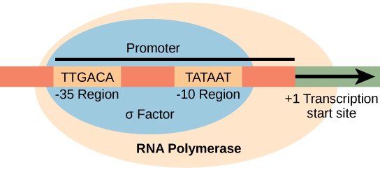
Figure 15.8 The σ subunit of prokaryotic RNA polymerase recognizes consensus sequences found in the promoter region upstream of the transcription start site. The σ subunit dissociates from the polymerase after transcription has been initiated.
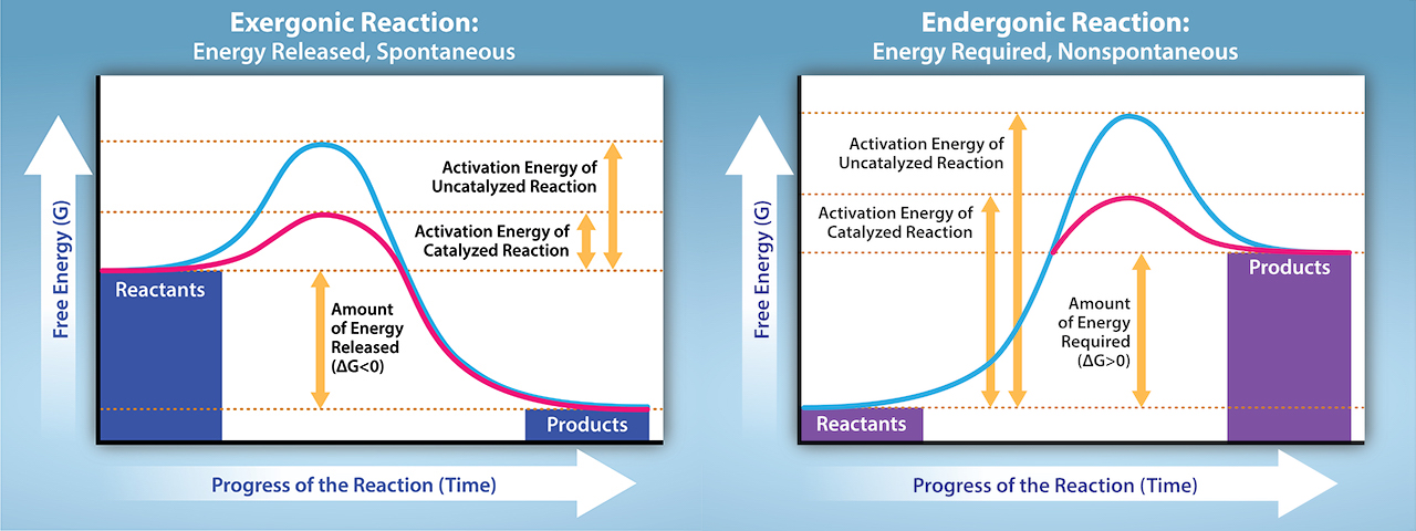
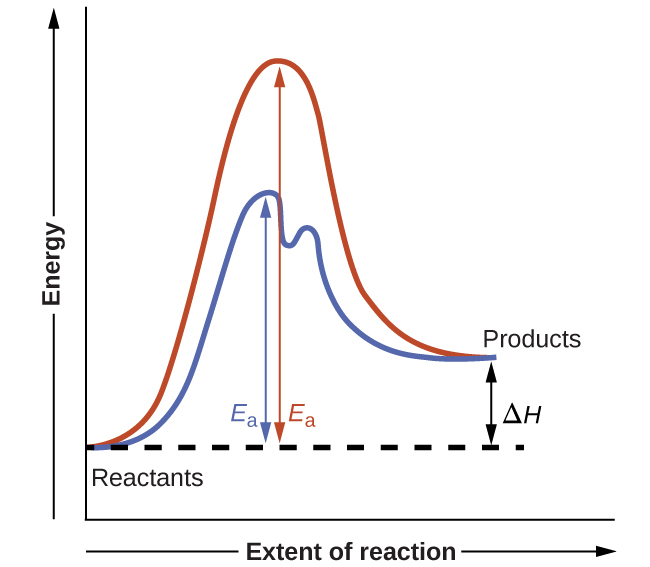
Figure 12.19 Reaction diagrams for an endothermic process in the absence (red curve) and presence (blue curve) of a catalyst. The catalyzed pathway involves a two-step mechanism (note the presence of two transition states) and an intermediate species (represented by the valley between the two transitions states).
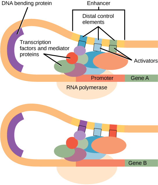
Figure 16.10 Interaction between proteins at the promoter and enhancer sites. An enhancer is a DNA sequence that promotes transcription. Each enhancer is made up of short DNA sequences called distal control elements. Activators bound to the distal control elements interact with mediator proteins and transcription factors. Two different genes may have the same promoter but different distal control elements, enabling differential gene expression.
Figure 15.8 The σ subunit of prokaryotic RNA polymerase recognizes consensus sequences found in the promoter region upstream of the transcription start site. The σ subunit dissociates from the polymerase after transcription has been initiated.
Figure 4.44 - Kinetic profile of an allosteric enzyme whose activity is controlled by a homotropic effector. Image by Aleia Kim
Kevin Ahern, Indira Rajagopal, and Taralyn Tan, Biochemistry Free For All, Oregon State University, via Biology LibreTexts. Image by Aleia Kim · CC BY-NC-SA 4.0
· Original image ↗ · Access for free ↗
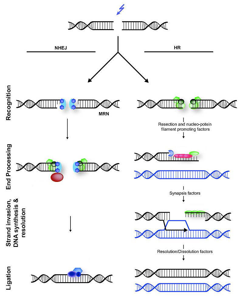
Figure 7.45 - Non-homologous end joining (left) versus homologous recombination (right) - Wikipedia
Wikipedia, as credited by Kevin Ahern, Indira Rajagopal, and Taralyn Tan, Biochemistry Free For All, Oregon State University, via Biology LibreTexts. · Source attribution
· Original image ↗ · Access for free ↗
The amount of a substance that can dissolve in a solvent under specified conditions. Soluble means able to dissolve; insoluble means only very slightly soluble in that solvent.
Figure 15.7 Messenger RNA is a copy of protein-coding information in the coding strand of DNA, with the substitution of U in the RNA for T in the coding sequence. However, new RNA nucleotides base pair with the nucleotides of the template strand. RNA is synthesized in its 5'-3' direction, using the enzyme RNA polymerase. As the template is read, the DNA unwinds ahead of the polymerase and then rewinds behind it.
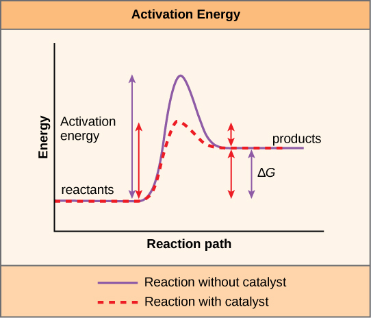
A fleeting, high-energy arrangement at a reaction barrier. It is an energy maximum along the reaction path, rather than a stable reaction intermediate.
Figure 12.19 Reaction diagrams for an endothermic process in the absence (red curve) and presence (blue curve) of a catalyst. The catalyzed pathway involves a two-step mechanism (note the presence of two transition states) and an intermediate species (represented by the valley between the two transitions states).
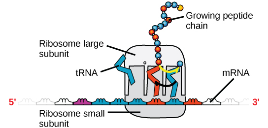
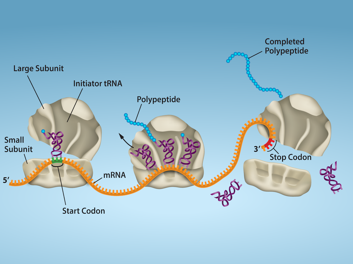
Figure 15.18 Translation begins when an initiator tRNA anticodon recognizes a start codon on mRNA bound to a small ribosomal subunit. The large ribosomal subunit joins the small subunit, and a second tRNA is recruited. As the mRNA moves relative to the ribosome, successive tRNAs move through the ribosome and the polypeptide chain is formed. Entry of a release factor into the A site terminates translation and the components dissociate.
Figure 4.21 - Kcat (turnover number) values for several enzymes. Image by Aleia Kim
Kevin Ahern, Indira Rajagopal, and Taralyn Tan, Biochemistry Free For All, Oregon State University, via Biology LibreTexts. Image by Aleia Kim · CC BY-NC-SA 4.0
· Original image ↗ · Access for free ↗
No matching terms. Try a different name or abbreviation.
2.2 Approaches to Research
OpenStax · 2.2 Approaches to Research ↗ Instructional page including learning objectives, examples, figures, source tables and questions. Site navigation and embedded media players are omitted; source media links remain available.
Learning Objectives
By the end of this section, you will be able to:
Describe the different research methods used by psychologists
Discuss the strengths and weaknesses of case studies, naturalistic observation, surveys, and archival research
Compare longitudinal and cross-sectional approaches to research
Compare and contrast correlation and causation
There are many research methods available to psychologists in their efforts to understand, describe, and explain behavior and the cognitive and biological processes that underlie it. Some methods rely on observational techniques. Other approaches involve interactions between the researcher and the individuals who are being studied—ranging from a series of simple questions to extensive, in-depth interviews—to well-controlled experiments.
Each of these research methods has unique strengths and weaknesses, and each method may only be appropriate for certain types of research questions. For example, studies that rely primarily on observation produce incredible amounts of information, but the ability to apply this information to the larger population is somewhat limited because of small sample sizes. Survey research, on the other hand, allows researchers to easily collect data from relatively large samples. While this allows for results to be generalized to the larger population more easily, the information that can be collected on any given survey is somewhat limited and subject to problems associated with any type of self-reported data. Some researchers conduct archival research by using existing records. While this can be a fairly inexpensive way to collect data that can provide insight into a number of research questions, researchers using this approach have no control on how or what kind of data was collected. All of the methods described thus far are correlational in nature. This means that researchers can speak to important relationships that might exist between two or more variables of interest. However, correlational data cannot be used to make claims about cause-and-effect relationships.
Correlational research can find a relationship between two variables, but the only way a researcher can claim that the relationship between the variables is cause and effect is to perform an experiment. In experimental research, which will be discussed later in this chapter, there is a tremendous amount of control over variables of interest. While this is a powerful approach, experiments are often conducted in artificial settings. This calls into question the validity of experimental findings with regard to how they would apply in real-world settings. In addition, many of the questions that psychologists would like to answer cannot be pursued through experimental research because of ethical concerns.
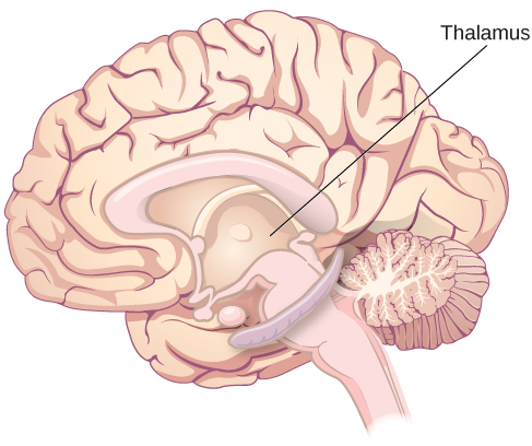
In 2011, the New York Times published a feature story on Krista and Tatiana Hogan, Canadian twin girls. These particular twins are unique because Krista and Tatiana are conjoined twins, connected at the head. There is evidence that the two girls are connected in a part of the brain called the thalamus, which is a major sensory relay center. Most incoming sensory information is sent through the thalamus before reaching higher regions of the cerebral cortex for processing.
The implications of this potential connection mean that it might be possible for one twin to experience the sensations of the other twin. For instance, if Krista is watching a particularly funny television program, Tatiana might smile or laugh even if she is not watching the program. This particular possibility has piqued the interest of many neuroscientists who seek to understand how the brain uses sensory information.
These twins represent an enormous resource in the study of the brain, and since their condition is very rare, it is likely that as long as their family agrees, scientists will follow these girls very closely throughout their lives to gain as much information as possible (Dominus, 2011).
Over time, it has become clear that while Krista and Tatiana share some sensory experiences and motor control, they remain two distinct individuals, which provides invaluable insight for researchers interested in the mind and the brain (Egnor, 2017).
In observational research, scientists are conducting a clinical or case study when they focus on one person or just a few individuals. Indeed, some scientists spend their entire careers studying just 10–20 individuals. Why would they do this? Obviously, when they focus their attention on a very small number of people, they can gain a precious amount of insight into those cases. The richness of information that is collected in clinical or case studies is unmatched by any other single research method. This allows the researcher to have a very deep understanding of the individuals and the particular phenomenon being studied.
If clinical or case studies provide so much information, why are they not more frequent among researchers? As it turns out, the major benefit of this particular approach is also a weakness. As mentioned earlier, this approach is often used when studying individuals who are interesting to researchers because they have a rare characteristic. Therefore, the individuals who serve as the focus of case studies are not like most other people. If scientists ultimately want to explain all behavior, focusing attention on such a special group of people can make it difficult to generalize any observations to the larger population as a whole. Generalizing refers to the ability to apply the findings of a particular research project to larger segments of society. Again, case studies provide enormous amounts of information, but since the cases are so specific, the potential to apply what’s learned to the average person may be very limited.
Naturalistic Observation
If you want to understand how behavior occurs, one of the best ways to gain information is to simply observe the behavior in its natural context. However, people might change their behavior in unexpected ways if they know they are being observed. How do researchers obtain accurate information when people tend to hide their natural behavior? As an example, imagine that your professor asks everyone in your class to raise their hand if they always wash their hands after using the restroom. Chances are that almost everyone in the classroom will raise their hand, but do you think hand washing after every trip to the restroom is really that universal?
This is very similar to the phenomenon mentioned earlier in this chapter: many individuals do not feel comfortable answering a question honestly. But if we are committed to finding out the facts about hand washing, we have other options available to us.
Suppose we send a classmate into the restroom to actually watch whether everyone washes their hands after using the restroom. Will our observer blend into the restroom environment by wearing a white lab coat, sitting with a clipboard, and staring at the sinks? We want our researcher to be inconspicuous—perhaps standing at one of the sinks pretending to put in contact lenses while secretly recording the relevant information. This type of observational study is called naturalistic observation: observing behavior in its natural setting. To better understand peer exclusion, Suzanne Fanger collaborated with colleagues at the University of Texas to observe the behavior of preschool children on a playground. How did the observers remain inconspicuous over the duration of the study? They equipped a few of the children with wireless microphones (which the children quickly forgot about) and observed while taking notes from a distance. Also, the children in that particular preschool (a “laboratory preschool”) were accustomed to having observers on the playground (Fanger, Frankel, & Hazen, 2012).
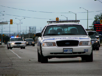
It is critical that the observer be as unobtrusive and as inconspicuous as possible: when people know they are being watched, they are less likely to behave naturally. If you have any doubt about this, ask yourself how your driving behavior might differ in two situations: In the first situation, you are driving down a deserted highway during the middle of the day; in the second situation, you are being followed by a police car down the same deserted highway (Figure 2.7).
Figure 2.7 — 2.2 Approaches to Research
Figure 2.7 Seeing a police car behind you would probably affect your driving behavior. (credit: Michael Gil)
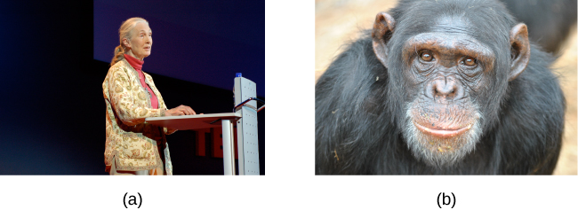
It should be pointed out that naturalistic observation is not limited to research involving humans. Indeed, some of the best-known examples of naturalistic observation involve researchers going into the field to observe various kinds of animals in their own environments. As with human studies, the researchers maintain their distance and avoid interfering with the animal subjects so as not to influence their natural behaviors. Scientists have used this technique to study social hierarchies and interactions among animals ranging from ground squirrels to gorillas. The information provided by these studies is invaluable in understanding how those animals organize socially and communicate with one another. The anthropologist Jane Goodall, for example, spent nearly five decades observing the behavior of chimpanzees in Africa (Figure 2.8). As an illustration of the types of concerns that a researcher might encounter in naturalistic observation, some scientists criticized Goodall for giving the chimps names instead of referring to them by numbers—using names was thought to undermine the emotional detachment required for the objectivity of the study (McKie, 2010).
Figure 2.8 — 2.2 Approaches to Research
Figure 2.8 (a) Jane Goodall made a career of conducting naturalistic observations of (b) chimpanzee behavior. (credit “Jane Goodall”: modification of work by Erik Hersman; “chimpanzee”: modification of work by “Afrika Force”/Flickr.com)
Rose M. Spielman, William J. Jenkins, and Marilyn D. Lovett, Psychology 2E, OpenStax. (credit “Jane Goodall”: modification of work by Erik Hersman; “chimpanzee”: modification of work by “Afrika Force”/Flickr.com) · CC BY-NC-SA 4.0
· Original image ↗ · Access for free ↗
The greatest benefit of naturalistic observation is the validity, or accuracy, of information collected unobtrusively in a natural setting. Having individuals behave as they normally would in a given situation means that we have a higher degree of ecological validity, or realism, than we might achieve with other research approaches. Therefore, our ability to generalize the findings of the research to real-world situations is enhanced. If done correctly, we need not worry about people or animals modifying their behavior simply because they are being observed. Sometimes, people may assume that reality programs give us a glimpse into authentic human behavior. However, the principle of inconspicuous observation is violated as reality stars are followed by camera crews and are interviewed on camera for personal confessionals. Given that environment, we must doubt how natural and realistic their behaviors are.
The major downside of naturalistic observation is that they are often difficult to set up and control. In our restroom study, what if you stood in the restroom all day prepared to record people’s hand washing behavior and no one came in? Or, what if you have been closely observing a troop of gorillas for weeks only to find that they migrated to a new place while you were sleeping in your tent? The benefit of realistic data comes at a cost. As a researcher you have no control of when (or if) you have behavior to observe. In addition, this type of observational research often requires significant investments of time, money, and a good dose of luck.
Sometimes studies involve structured observation. In these cases, people are observed while engaging in set, specific tasks. An excellent example of structured observation comes from Strange Situation by Mary Ainsworth (you will read more about this in the chapter on lifespan development). The Strange Situation is a procedure used to evaluate attachment styles that exist between an infant and caregiver. In this scenario, caregivers bring their infants into a room filled with toys. The Strange Situation involves a number of phases, including a stranger coming into the room, the caregiver leaving the room, and the caregiver’s return to the room. The infant’s behavior is closely monitored at each phase, but it is the behavior of the infant upon being reunited with the caregiver that is most telling in terms of characterizing the infant’s attachment style with the caregiver.
Another potential problem in observational research is observer bias. Generally, people who act as observers are closely involved in the research project and may unconsciously skew their observations to fit their research goals or expectations. To protect against this type of bias, researchers should have clear criteria established for the types of behaviors recorded and how those behaviors should be classified. In addition, researchers often compare observations of the same event by multiple observers, in order to test inter-rater reliability: a measure of reliability that assesses the consistency of observations by different observers.
Surveys
Often, psychologists develop surveys as a means of gathering data. Surveys are lists of questions to be answered by research participants, and can be delivered as paper-and-pencil questionnaires, administered electronically, or conducted verbally (Figure 2.9). Generally, the survey itself can be completed in a short time, and the ease of administering a survey makes it easy to collect data from a large number of people.
Surveys allow researchers to gather data from larger samples than may be afforded by other research methods. A sample is a subset of individuals selected from a population, which is the overall group of individuals that the researchers are interested in. Researchers study the sample and seek to generalize their findings to the population. Generally, researchers will begin this process by calculating various measures of central tendency from the data they have collected. These measures provide an overall summary of what a typical response looks like. There are three measures of central tendency: mode, median, and mean. The mode is the most frequently occurring response, the median lies at the middle of a given data set, and the mean is the arithmetic average of all data points. Means tend to be most useful in conducting additional analyses like those described below; however, means are very sensitive to the effects of outliers, and so one must be aware of those effects when making assessments of what measures of central tendency tell us about a data set in question.
Figure 2.9 — 2.2 Approaches to Research
Figure 2.9 Surveys can be administered in a number of ways, including electronically administered research, like the survey shown here. (credit: Robert Nyman)
There is both strength and weakness of the survey in comparison to case studies. By using surveys, we can collect information from a larger sample of people. A larger sample is better able to reflect the actual diversity of the population, thus allowing better generalizability. Therefore, if our sample is sufficiently large and diverse, we can assume that the data we collect from the survey can be generalized to the larger population with more certainty than the information collected through a case study. However, given the greater number of people involved, we are not able to collect the same depth of information on each person that would be collected in a case study.
Another potential weakness of surveys is something we touched on earlier in this chapter: People don't always give accurate responses. They may lie, misremember, or answer questions in a way that they think makes them look good. For example, people may report drinking less alcohol than is actually the case.
Any number of research questions can be answered through the use of surveys. One real-world example is the research conducted by Jenkins, Ruppel, Kizer, Yehl, and Griffin (2012) about the backlash against the US Arab-American community following the terrorist attacks of September 11, 2001. Jenkins and colleagues wanted to determine to what extent these negative attitudes toward Arab-Americans still existed nearly a decade after the attacks occurred. In one study, 140 research participants filled out a survey with 10 questions, including questions asking directly about the participant’s overt prejudicial attitudes toward people of various ethnicities. The survey also asked indirect questions about how likely the participant would be to interact with a person of a given ethnicity in a variety of settings (such as, “How likely do you think it is that you would introduce yourself to a person of Arab-American descent?”). The results of the research suggested that participants were unwilling to report prejudicial attitudes toward any ethnic group. However, there were significant differences between their pattern of responses to questions about social interaction with Arab-Americans compared to other ethnic groups: they indicated less willingness for social interaction with Arab-Americans compared to the other ethnic groups. This suggested that the participants harbored subtle forms of prejudice against Arab-Americans, despite their assertions that this was not the case (Jenkins et al., 2012).
Archival Research
Some researchers gain access to large amounts of data without interacting with a single research participant. Instead, they use existing records to answer various research questions. This type of research approach is known as archival research. Archival research relies on looking at past records or data sets to look for interesting patterns or relationships.
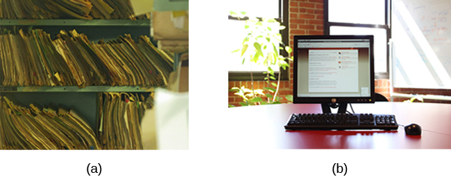
For example, a researcher might access the academic records of all individuals who enrolled in college within the past ten years and calculate how long it took them to complete their degrees, as well as course loads, grades, and extracurricular involvement. Archival research could provide important information about who is most likely to complete their education, and it could help identify important risk factors for struggling students (Figure 2.10).
Figure 2.10 — 2.2 Approaches to Research
Figure 2.10 A researcher doing archival research examines records, whether archived as a (a) hardcopy or (b) electronically. (credit “paper files”: modification of work by “Newtown graffiti”/Flickr; “computer”: modification of work by INPIVIC Family/Flickr)
Rose M. Spielman, William J. Jenkins, and Marilyn D. Lovett, Psychology 2E, OpenStax. (credit “paper files”: modification of work by “Newtown graffiti”/Flickr; “computer”: modification of work by INPIVIC Family/Flickr) · CC BY-NC-SA 4.0
· Original image ↗ · Access for free ↗
In comparing archival research to other research methods, there are several important distinctions. For one, the researcher employing archival research never directly interacts with research participants. Therefore, the investment of time and money to collect data is considerably less with archival research. Additionally, researchers have no control over what information was originally collected. Therefore, research questions have to be tailored so they can be answered within the structure of the existing data sets. There is also no guarantee of consistency between the records from one source to another, which might make comparing and contrasting different data sets problematic.
Longitudinal and Cross-Sectional Research
Sometimes we want to see how people change over time, as in studies of human development and lifespan. When we test the same group of individuals repeatedly over an extended period of time, we are conducting longitudinal research. Longitudinal research is a research design in which data-gathering is administered repeatedly over an extended period of time. For example, we may survey a group of individuals about their dietary habits at age 20, retest them a decade later at age 30, and then again at age 40.
Another approach is cross-sectional research. In cross-sectional research, a researcher compares multiple segments of the population at the same time. Using the dietary habits example above, the researcher might directly compare different groups of people by age. Instead of studying a group of people for 20 years to see how their dietary habits changed from decade to decade, the researcher would study a group of 20-year-old individuals and compare them to a group of 30-year-old individuals and a group of 40-year-old individuals. While cross-sectional research requires a shorter-term investment, it is also limited by differences that exist between the different generations (or cohorts) that have nothing to do with age per se, but rather reflect the social and cultural experiences of different generations of individuals that make them different from one another.
To illustrate this concept, consider the following survey findings. In recent years there has been significant growth in the popular support of same-sex marriage. Many studies on this topic break down survey participants into different age groups. In general, younger people are more supportive of same-sex marriage than are those who are older (Jones, 2013). Does this mean that as we age we become less open to the idea of same-sex marriage, or does this mean that older individuals have different perspectives because of the social climates in which they grew up? Longitudinal research is a powerful approach because the same individuals are involved in the research project over time, which means that the researchers need to be less concerned with differences among cohorts affecting the results of their study.
Often longitudinal studies are employed when researching various diseases in an effort to understand particular risk factors. Such studies often involve tens of thousands of individuals who are followed for several decades. Given the enormous number of people involved in these studies, researchers can feel confident that their findings can be generalized to the larger population. The Cancer Prevention Study-3 (CPS-3) is one of a series of longitudinal studies sponsored by the American Cancer Society aimed at determining predictive risk factors associated with cancer. When participants enter the study, they complete a survey about their lives and family histories, providing information on factors that might cause or prevent the development of cancer. Then every few years the participants receive additional surveys to complete. In the end, hundreds of thousands of participants will be tracked over 20 years to determine which of them develop cancer and which do not.
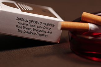
Clearly, this type of research is important and potentially very informative. For instance, earlier longitudinal studies sponsored by the American Cancer Society provided some of the first scientific demonstrations of the now well-established links between increased rates of cancer and smoking (American Cancer Society, n.d.) (Figure 2.11).
Figure 2.11 — 2.2 Approaches to Research
Figure 2.11 Longitudinal research like the CPS-3 help us to better understand how smoking is associated with cancer and other diseases. (credit: CDC/Debora Cartagena)
As with any research strategy, longitudinal research is not without limitations. For one, these studies require an incredible time investment by the researcher and research participants. Given that some longitudinal studies take years, if not decades, to complete, the results will not be known for a considerable period of time. In addition to the time demands, these studies also require a substantial financial investment. Many researchers are unable to commit the resources necessary to see a longitudinal project through to the end.
Research participants must also be willing to continue their participation for an extended period of time, and this can be problematic. People move, get married and take new names, get ill, and eventually die. Even without significant life changes, some people may simply choose to discontinue their participation in the project. As a result, the attrition rates, or reduction in the number of research participants due to dropouts, in longitudinal studies are quite high and increase over the course of a project. For this reason, researchers using this approach typically recruit many participants fully expecting that a substantial number will drop out before the end. As the study progresses, they continually check whether the sample still represents the larger population, and make adjustments as necessary.
9.4 Rare Events, the Sample, Decision and Conclusion
Establishing the type of distribution, sample size, and known or unknown standard deviation can help you figure out how to go about a hypothesis test. However, there are several other factors you should consider when working out a hypothesis test.
Rare Events
Suppose you make an assumption about a property of the population (this assumption is the null hypothesis). Then you gather sample data randomly. If the sample has properties that would be very unlikely to occur if the assumption is true, then you would conclude that your assumption about the population is probably incorrect. (Remember that your assumption is just an assumption—it is not a fact and it may or may not be true. But your sample data are real and the data are showing you a fact that seems to contradict your assumption.)
For example, Didi and Ali are at a birthday party of a very wealthy friend. They hurry to be first in line to grab a prize from a tall basket that they cannot see inside because they will be blindfolded. There are 200 plastic bubbles in the basket and Didi and Ali have been told that there is only one with a $100 bill. Didi is the first person to reach into the basket and pull out a bubble. Her bubble contains a $100 bill. The probability of this happening is = 0.005. Because this is so unlikely, Ali is hoping that what the two of them were told is wrong and there are more $100 bills in the basket. A "rare event" has occurred (Didi getting the $100 bill) so Ali doubts the assumption about only one $100 bill being in the basket.
Use the sample data to calculate the actual probability of getting the test result, called the p-value. The p-value is the probability that, if the null hypothesis is true, the results from another randomly selected sample will be as extreme or more extreme as the results obtained from the given sample.
A large p-value calculated from the data indicates that we should not reject the null hypothesis. The smaller the p-value, the more unlikely the outcome, and the stronger the evidence is against the null hypothesis. We would reject the null hypothesis if the evidence is strongly against it.
Draw a graph that shows the p-value. The hypothesis test is easier to perform if you use a graph because you see the problem more clearly.
Example
9.9
Suppose a baker claims that his bread height is more than 15 cm, on average. Several of his customers do not believe him. To persuade his customers that he is right, the baker decides to do a hypothesis test. He bakes 10 loaves of bread. The mean height of the sample loaves is 17 cm. The baker knows from baking hundreds of loaves of bread that the standard deviation for the height is 0.5 cm. and the distribution of heights is normal.
The null hypothesis could be H0: μ ≤ 15 The alternate hypothesis is Ha: μ > 15
The words "is more than" translates as a ">" so "μ > 15" goes into the alternate hypothesis. The null hypothesis must contradict the alternate hypothesis.
By the Central Limit Theorem, the distribution of sample means, for samples of 10 loaves, will be normal with mean μ = 15 and standard deviation .
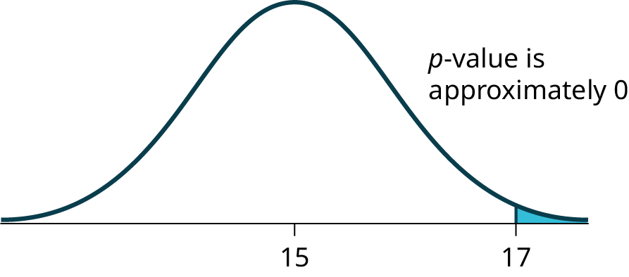
Suppose the null hypothesis is true (the mean height of the loaves is no more than 15 cm). Then is the mean height (17 cm) calculated from the sample unexpectedly large? The hypothesis test works by asking the question how unlikely the sample mean would be if the null hypothesis were true. The graph shows how far out the sample mean is on the normal curve. The p-value is the probability that, if we were to take other samples, any other sample mean would fall at least as far out as 17 cm.
The p-value, then, is the probability that a sample mean is the same or greater than 17 cm. when the population mean is, in fact, 15 cm. We can calculate this probability using the normal distribution for means.
Figure 9.2 — 9.4 Rare Events, the Sample, Decision and Conclusion
A p-value of approximately zero tells us that it is highly unlikely that a loaf of bread rises no more than 15 cm, on average. That is, almost 0% of all loaves of bread would be at least as high as 17 cm. purely by CHANCE had the population mean height really been 15 cm. Because the outcome of 17 cm. is so unlikely (meaning it is happening NOT by chance alone), we conclude that the evidence is strongly against the null hypothesis (the mean height is at most 15 cm.). There is sufficient evidence that the true mean height for the population of the baker's loaves of bread is greater than 15 cm.
Try It
9.9
A normal distribution has a standard deviation of 1. We want to verify a claim that the mean is greater than 12. A sample of 36 is taken with a sample mean of 12.5.
H0: μ ≤ 12
Ha: μ > 12
The p-value is 0.0013
Draw a graph that shows the p-value.
Decision and Conclusion
A systematic way to make a decision of whether to reject or not reject the null hypothesis
is to compare the p-value and a preset or preconceived α (also called a "significance level"). A preset α is the probability of a Type I error (rejecting the null hypothesis when the null hypothesis is true). It may or may not be given to you at the beginning of the problem.
When you make a decision to reject or not reject H0, do as follows:
If α > p-value, reject H0. The results of the sample data are significant. There is sufficient evidence to conclude that H0 is an incorrect belief and that the alternative hypothesis, Ha, may be correct.
If α ≤ p-value, do not reject H0. The results of the sample data are not significant.There is not sufficient evidence to conclude that the alternative hypothesis,Ha, may be correct.
When you "do not reject H0", it does not mean that you should believe that H0 is true. It simply means that the sample data have failed to provide sufficient evidence to cast serious doubt about the truthfulness of Ho.
Conclusion: After you make your decision, write a thoughtful conclusion about the hypotheses in terms of the given problem.
Example
9.10
When using the p-value to evaluate a hypothesis test, it is sometimes useful to use the following memory device
If the p-value is low, the null must go.
If the p-value is high, the null must fly.
This memory aid relates a p-value less than the established alpha (the p is low) as rejecting the null hypothesis and, likewise, relates a p-value higher than the established alpha (the p is high) as not rejecting the null hypothesis.
Problem
Fill in the blanks.
Reject the null hypothesis when ______________________________________.
The results of the sample data _____________________________________.
Do not reject the null when hypothesis when __________________________________________.
The results of the sample data ____________________________________________.
Reject the null hypothesis when the p-value is less than the established alpha value. The results of the sample data support the alternative hypothesis.
Do not reject the null hypothesis when the p-value is greater than the established alpha value. The results of the sample data do not support the alternative hypothesis.
Try It
9.10
It’s a Boy Genetics Labs claim their procedures improve the chances of a boy being born. The results for a test of a single population proportion are as follows:
H0: p = 0.50, Ha: p > 0.50
α = 0.01
p-value = 0.025
Interpret the results and state a conclusion in simple, non-technical terms.
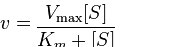
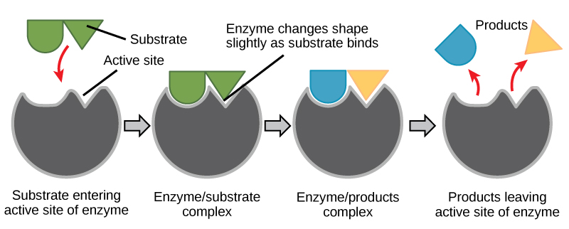
To understand how an enzyme enhances the rate of a reaction, we must understand enzymekinetics. We present a model here proposed by Leonor Michaelis and Maud Menten. In order to understand the model, it is necessary to understand a few parameters.
First, we describe a reaction in simple terms proceeding as follows
where ES* is the activated state and EP is the enzyme-product complex before release of the product.
The first consideration we have is velocity. The velocity of a reaction is the rate of creation of product over time, measured as the concentration of product per time. The time is a critical consideration when measuring velocity. In a closed system (in which an enzyme operates), all reactions will advance towards equilibrium. Enzymatically catalyzed reactions are no different in the end result from non-enzymatic reactions, except that they get to equilibrium faster.
Experimental considerations
Now we turn our attention to how studies of the kinetic properties of an enzyme are conducted. To perform an analysis, one would do the following experiment - 20 different tubes would be set up with enzymebuffer (to keep the enzyme stable), the same amount of enzyme, and then a different amount of substrate in each tube, ranging from tiny amounts in the first tubes to very large amounts in the last tubes. The reaction would be allowed to proceed for a fixed, short amount of time and then the reaction would be stopped and the amount of product contained in each tube would be determined.
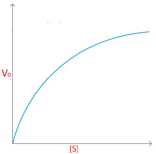
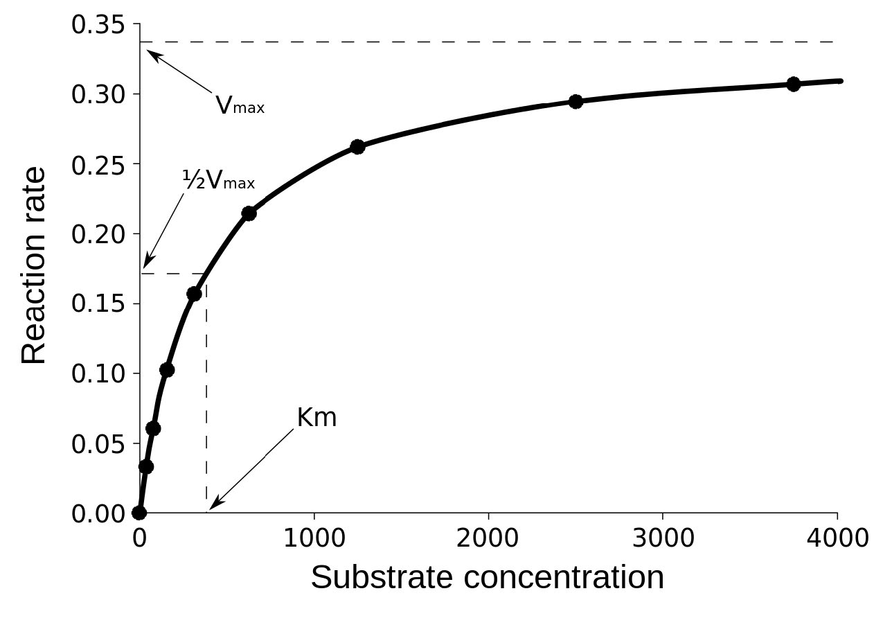
On a plot of initial velocity versus substrate concentration (V0 vs. [S]), Vmax is the value on the Y axis that the curve asymptotically approaches (dotted line in Figure 4.20). It should be noted that the value of Vmax depends on the amount of enzyme used in a reaction. If you double the amount of enzyme used, you will double the Vmax. If one wanted to compare the velocities of two different enzymes, it would be necessary to use the same amounts of enzyme in the reaction each one catalyzes.
Affinities of enzymes for substrates vary considerably, so knowing Km helps us to understand how well an enzyme is suited to the substrate being used. Measurement of Km depends on the measurement of Vmax.
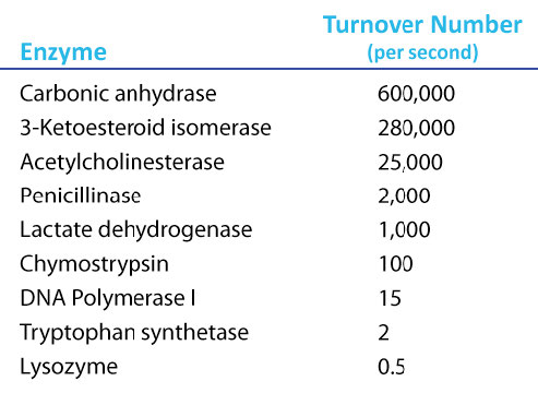
Figure 4.21 - Kcat (turnover number) values for several enzymes. Image by Aleia Kim
Kevin Ahern, Indira Rajagopal, and Taralyn Tan, Biochemistry Free For All, Oregon State University, via Biology LibreTexts. Image by Aleia Kim · CC BY-NC-SA 4.0
· Original image ↗ · Access for free ↗
A kcat value of 1000 molecules of product per enzyme per second might seem like a high value, but there are enzymes known (carbonic anhydrase, for example) that have a kcat value of over 600,000/second (Figure 4.21). This astonishing value illustrates clearly why enzymes seem almost magical in their action. In contrast to , which varies with the amount of enzyme used, kcat is a constant for an enzyme under given conditions.
Why should there be a maximum possible value of Kcat / Km? The answer is that movement of substrate to the enzyme becomes the limiting factor for perfect enzymes. Movement of substrate by diffusion in water has a fixed rate at any temperature and that limitation ultimately determines the maximum speed an enzyme can catalyze at. In a macroscopic world analogy, factories can’t make products faster than suppliers can deliver materials. It is safe to say for a perfect enzyme that the only speed limit it has is the rate of substratediffusion in water.
Given the “magic” of enzymes alluded to earlier, it might seem that all enzymes should have evolved to be “perfect.” There are very good reasons why most of them have not.
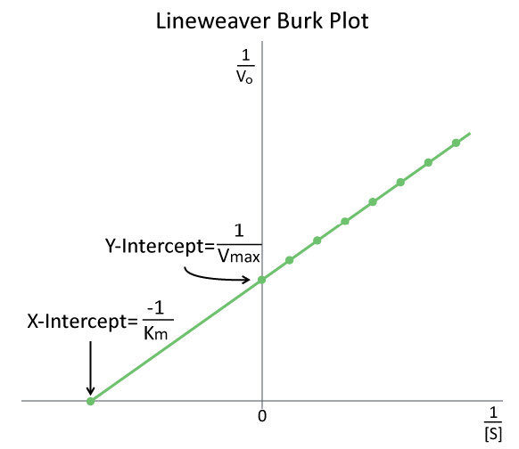
The study of enzymekinetics is typically the most math intensive component of biochemistry and one of the most daunting aspects of the subject for many students. Although attempts are made to simplify the mathematical considerations, sometimes they only serve to confuse or frustrate students. Such is the case with modified enzyme plots, such as Lineweaver-Burk (Figure 4.26).
Indeed, when presented by professors as simply another thing to memorize, who can blame students? In reality, both of these plots are aimed at simplifying the determination of parameters, such as and . In making either of these modified plots, it is important to recognize that the same data is used as in making a V0 vs. [S] plot. The data are simply manipulated to make the plotting easier.
Figure 4.26 - A Lineweaver-Burk plot of 1/V₀ vs 1/[S]. Image by Aleia Kim
Kevin Ahern, Indira Rajagopal, and Taralyn Tan, Biochemistry Free For All, Oregon State University, via Biology LibreTexts. Image by Aleia Kim · CC BY-NC-SA 4.0
· Original image ↗ · Access for free ↗
Double reciprocal
For a LineWeaver-Burk plot, the manipulation is using the reciprocal of the values of both the velocity and the substrate concentration. The inverted values are then plotted on a graph as 1/V0 vs. 1/[S]. Because of these inversions, Lineweaver-Burk plots are commonly referred to as ‘double-reciprocal’ plots. As can be seen in Figure 4.26, the value of Km on a Lineweaver Burk plot is easily determined as the negative reciprocal of the x-intercept , whereas the Vmax is the inverse of the y-intercept. Other related manipulation of kinetic data include Eadie-Hofstee diagrams, which plots V0 vs V0/[S] and gives Vmax as the Y-axis intercept with the slope of the line being -Km.