Describe the observed comparison before deciding whether it supports an effect, a mechanism, or a generalization.
Read the encoding before the trend
Check variables, units, axis direction, linear versus logarithmic spacing, reference groups, and legend. A truncated vertical axis can visually amplify differences. Histograms describe distributions of numerical observations; bar plots often compare category summaries; scatterplots show paired measurements. Error bars require a definition: standard deviation, standard error, and confidence interval answer different questions. A line connecting means does not establish that each individual followed the same trajectory. A table can reveal sample sizes or baseline differences that a compact graph conceals.
Mean is the sum divided by count; median is the middle ordered observation; mode is the most frequent value. Range is maximum minus minimum; interquartile range spans the middle half of ordered values. Standard deviation measures dispersion around the mean in the original units. Outliers can move the mean and inflate range and standard deviation substantially; median and interquartile range are more resistant. Standard error describes sampling variability of an estimator, not variation among individual observations.
Random error varies unpredictably across repeated measurements; systematic error shifts results in a consistent way. Replication can reduce uncertainty in a mean without eliminating calibration bias. A frequentist 95% confidence-interval procedure covers the fixed true parameter in 95% of repeated samples under its assumptions; it does not give a 95% probability that this already computed interval contains the parameter. A p value is the probability, under a specified null model, of data at least as incompatible as observed. It is neither the probability the null is true nor a measure of practical importance.
Correlation summarizes association, which can arise from causation, reverse causation, confounding, or selection. Temporal order, intervention, consistent comparisons, and replication can strengthen a causal argument. A nonsignificant result may reflect low precision and does not prove equivalence; an equivalence claim needs an appropriate design and margin. Replication is expected to show compatible effects within uncertainty, not identical values. Separate an observed difference from the proposed mechanism and from extrapolation to populations, doses, or durations not studied.
Question. Group A has values 2, 3, 3, 4, 18. Compute mean, median, mode, and range. A different randomized study reports a small effect with p = 0.01: what does that establish, and what remains to assess?
Show reasoning
Mean = 30/5 = 6; median = 3; mode = 3; range = 18−2 = 16. The high outlier pulls the mean above the typical central values. With the stated null model, p = 0.01 means results at least this incompatible would occur with probability 0.01; it does not mean a 99% chance the mechanism is correct. Assess effect size, confidence interval, design quality, multiple comparisons, and practical relevance.
1.2 Data, Sampling, and Variation in Data and Sampling — figures and tables
Figure 1.3 — 1.2 Data, Sampling, and Variation in Data and Sampling
Figure 1.3
Barbara Illowsky and Susan Dean, Introductory Statistics 2E, OpenStax. · CC BY-NC-SA 4.0
· Original image ↗ · Access for free ↗Figure 1.4 — 1.2 Data, Sampling, and Variation in Data and Sampling
Figure 1.4
Barbara Illowsky and Susan Dean, Introductory Statistics 2E, OpenStax. · CC BY-NC-SA 4.0
· Original image ↗ · Access for free ↗Figure 1.5 — 1.2 Data, Sampling, and Variation in Data and Sampling
Figure 1.5
Barbara Illowsky and Susan Dean, Introductory Statistics 2E, OpenStax. · CC BY-NC-SA 4.0
· Original image ↗ · Access for free ↗Figure 1.6 — 1.2 Data, Sampling, and Variation in Data and Sampling
Figure 1.6
Barbara Illowsky and Susan Dean, Introductory Statistics 2E, OpenStax. · CC BY-NC-SA 4.0
· Original image ↗ · Access for free ↗Figure 1.7 — 1.2 Data, Sampling, and Variation in Data and Sampling
Figure 1.7
Barbara Illowsky and Susan Dean, Introductory Statistics 2E, OpenStax. · CC BY-NC-SA 4.0
· Original image ↗ · Access for free ↗Figure 1.8 — 1.2 Data, Sampling, and Variation in Data and Sampling
Figure 1.8
Barbara Illowsky and Susan Dean, Introductory Statistics 2E, OpenStax. · CC BY-NC-SA 4.0
· Original image ↗ · Access for free ↗Figure 1.9 — 1.2 Data, Sampling, and Variation in Data and Sampling
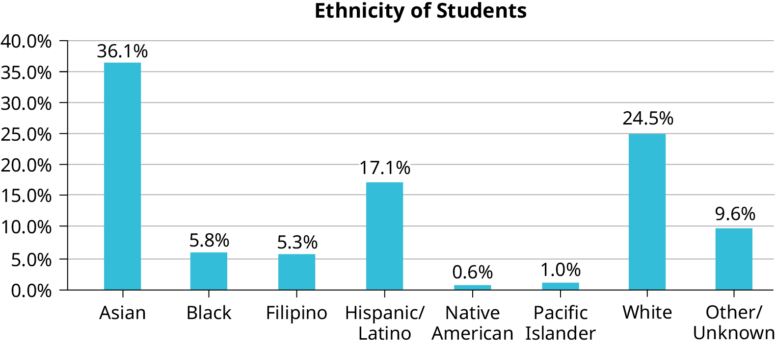
Figure 1.9 Bar Graph with Other/Unknown Category
Barbara Illowsky and Susan Dean, Introductory Statistics 2E, OpenStax. · CC BY-NC-SA 4.0
· Original image ↗ · Access for free ↗Figure 1.10 — 1.2 Data, Sampling, and Variation in Data and Sampling
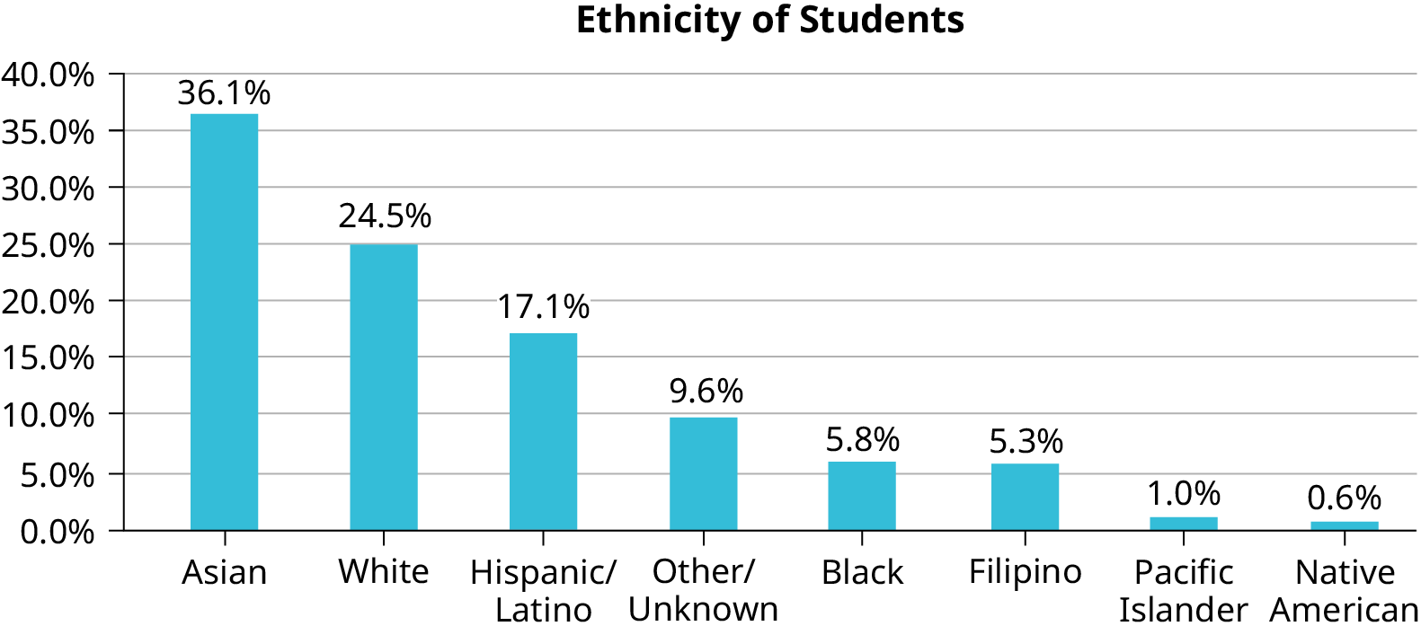
Figure 1.10 Pareto Chart With Bars Sorted by Size
Barbara Illowsky and Susan Dean, Introductory Statistics 2E, OpenStax. · CC BY-NC-SA 4.0
· Original image ↗ · Access for free ↗Figure 1.11 — 1.2 Data, Sampling, and Variation in Data and Sampling
Figure 1.11
Barbara Illowsky and Susan Dean, Introductory Statistics 2E, OpenStax. · CC BY-NC-SA 4.0
· Original image ↗ · Access for free ↗Figure 1.12 — 1.2 Data, Sampling, and Variation in Data and Sampling
Table 1.3 Most Recent Spring Quarter. Barbara Illowsky and Susan Dean, Introductory Statistics 2E, OpenStax.
Characteristic/Category
Percent
Full-Time Students
40.9%
Students who intend to transfer to a 4-year educational institution
48.6%
Students under age 25
61.0%
TOTAL
150.5%
Table 1.4 De Anza College Most Recent Spring Quarter. Barbara Illowsky and Susan Dean, Introductory Statistics 2E, OpenStax.
Frequency
Percent
Asian
8,794
36.1%
Black
1,412
5.8%
Filipino
1,298
5.3%
Hispanic/Latino
4,180
17.1%
Native American
146
0.6%
Pacific Islander
236
1.0%
White
5,978
24.5%
TOTAL
22,044 out of 24,382
90.4% out of 100%
Table 1.5 Ethnicity of Students at De Anza College in the Most Recent Fall Term. Barbara Illowsky and Susan Dean, Introductory Statistics 2E, OpenStax.
ID
Name
ID
Name
ID
Name
00
Anselmo
11
King
21
Roquero
01
Bautista
12
Legeny
22
Roth
02
Bayani
13
Lundquist
23
Rowell
03
Cheng
14
Macierz
24
Salangsang
04
Cuarismo
15
Motogawa
25
Slade
05
Cuningham
16
Okimoto
26
Stratcher
06
Fontecha
17
Patel
27
Tallai
07
Hong
18
Price
28
Tran
08
Hoobler
19
Quizon
29
Wai
09
Jiao
20
Reyes
30
Wood
10
Khan
Table 1.6 Class Roster. Barbara Illowsky and Susan Dean, Introductory Statistics 2E, OpenStax.
#1
#2
#3
#4
#5
#6
5
7
10
9
8
3
10
5
9
8
7
6
9
10
8
6
7
9
9
10
10
9
8
9
7
8
9
5
7
4
9
9
9
10
8
7
7
7
10
9
8
8
8
8
9
10
8
8
9
7
8
7
7
8
8
8
10
9
8
7
Table 1.7. Barbara Illowsky and Susan Dean, Introductory Statistics 2E, OpenStax.
Face on Die
Frequency
1
2
3
4
5
6
Table 1.8 First Experiment (20 rolls). Barbara Illowsky and Susan Dean, Introductory Statistics 2E, OpenStax.
Face on Die
Frequency
1
2
3
4
5
6
Table 1.9 Second Experiment (20 rolls). Barbara Illowsky and Susan Dean, Introductory Statistics 2E, OpenStax.
8.1 A Single Population Mean using the Normal Distribution — figures and tables
Figure 8.2 — 8.1 A Single Population Mean using the Normal Distribution
Figure 8.2
Barbara Illowsky and Susan Dean, Introductory Statistics 2E, OpenStax. · CC BY-NC-SA 4.0
· Original image ↗ · Access for free ↗Figure 8.3 — 8.1 A Single Population Mean using the Normal Distribution
Figure 8.3
Barbara Illowsky and Susan Dean, Introductory Statistics 2E, OpenStax. · CC BY-NC-SA 4.0
· Original image ↗ · Access for free ↗Figure 8.4 — 8.1 A Single Population Mean using the Normal Distribution
Figure 8.4
Barbara Illowsky and Susan Dean, Introductory Statistics 2E, OpenStax. · CC BY-NC-SA 4.0
· Original image ↗ · Access for free ↗Figure 8.5 — 8.1 A Single Population Mean using the Normal Distribution
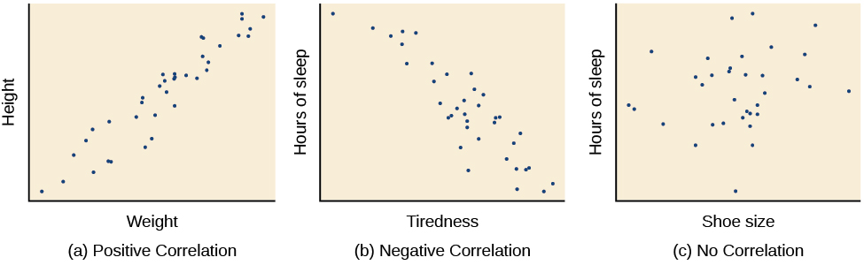
Figure 2.12 Scatterplots are a graphical view of the strength and direction of correlations. The stronger the correlation, the closer the data points are to a straight line. In these examples, we see that there is (a) a positive correlation between weight and height, (b) a negative correlation between tiredness and hours of sleep, and (c) no correlation between shoe size and hours of sleep.
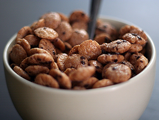
Figure 2.13 Does eating cereal really cause someone to be healthier? (credit: Tim Skillern)
Rose M. Spielman, William J. Jenkins, and Marilyn D. Lovett, Psychology 2E, OpenStax. (credit: Tim Skillern) · CC BY-NC-SA 4.0
· Original image ↗ · Access for free ↗Figure 2.14 — 2.3 Analyzing Findings
Figure 2.14 Many people believe that a full moon makes people behave oddly. (credit: Cory Zanker)
Rose M. Spielman, William J. Jenkins, and Marilyn D. Lovett, Psychology 2E, OpenStax. (credit: Cory Zanker) · CC BY-NC-SA 4.0
· Original image ↗ · Access for free ↗Figure 2.15 — 2.3 Analyzing Findings
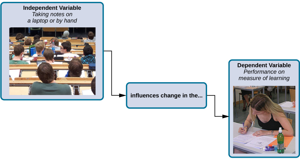
Figure 2.15 How might the use of technology in the classroom impact learning? (credit: modification of work by Nikolay Georgiev/Pixabay)
Rose M. Spielman, William J. Jenkins, and Marilyn D. Lovett, Psychology 2E, OpenStax. (credit: modification of work by Nikolay Georgiev/Pixabay) · CC BY-NC-SA 4.0
· Original image ↗ · Access for free ↗Figure 2.16 — 2.3 Analyzing Findings
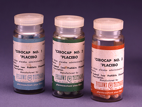
Figure 2.16 Providing the control group with a placebo treatment protects against bias caused by expectancy. (credit: Elaine and Arthur Shapiro)
Rose M. Spielman, William J. Jenkins, and Marilyn D. Lovett, Psychology 2E, OpenStax. (credit: Elaine and Arthur Shapiro) · CC BY-NC-SA 4.0
· Original image ↗ · Access for free ↗Figure 2.17 — 2.3 Analyzing Findings
Figure 2.17 In an experiment, manipulations of the independent variable are expected to result in changes in the dependent variable. (credit: “classroom” modification of work by Nikolay Georgiev/Pixabay; credit “note taking”: modification of work by KF/Wikimedia)
Rose M. Spielman, William J. Jenkins, and Marilyn D. Lovett, Psychology 2E, OpenStax. (credit: “classroom” modification of work by Nikolay Georgiev/Pixabay; credit “note taking”: modification of work by KF/Wikimedia) · CC BY-NC-SA 4.0
· Original image ↗ · Access for free ↗Figure 2.18 — 2.3 Analyzing Findings
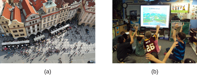
Figure 2.18 Researchers may work with (a) a large population or (b) a sample group that is a subset of the larger population. (credit “crowd”: modification of work by James Cridland; credit “students”: modification of work by Laurie Sullivan)
Rose M. Spielman, William J. Jenkins, and Marilyn D. Lovett, Psychology 2E, OpenStax. (credit “crowd”: modification of work by James Cridland; credit “students”: modification of work by Laurie Sullivan) · CC BY-NC-SA 4.0
· Original image ↗ · Access for free ↗Figure 2.19 — 2.3 Analyzing Findings
Figure 2.19 Some people still think vaccinations cause autism. (credit: modification of work by UNICEF Sverige)
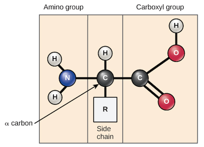
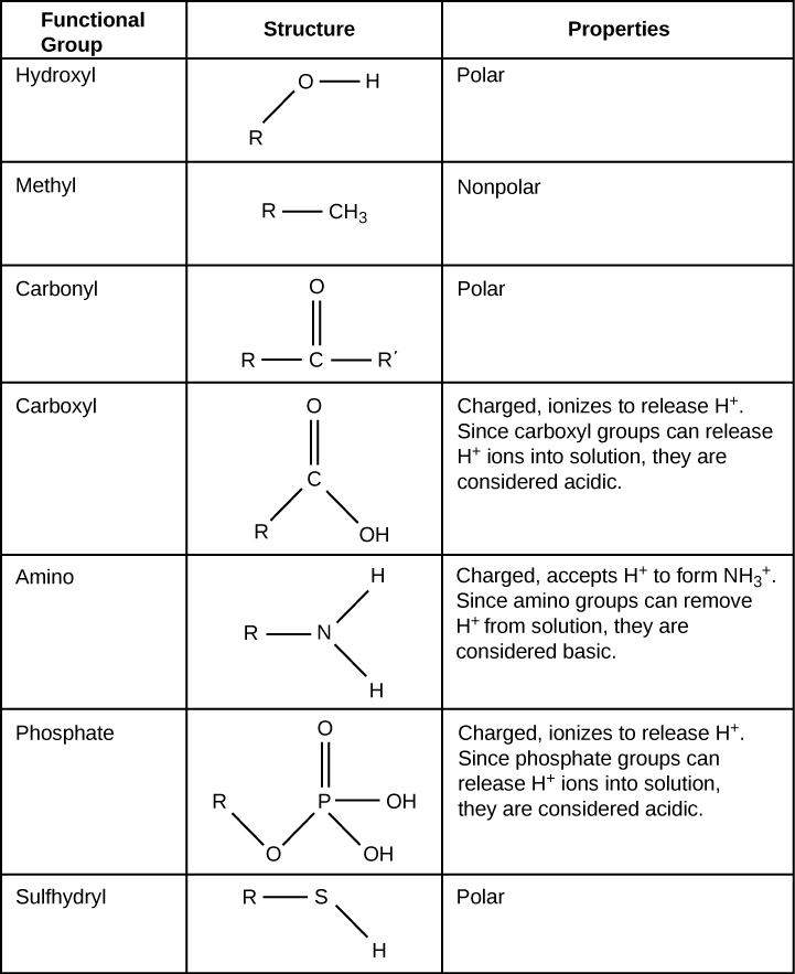
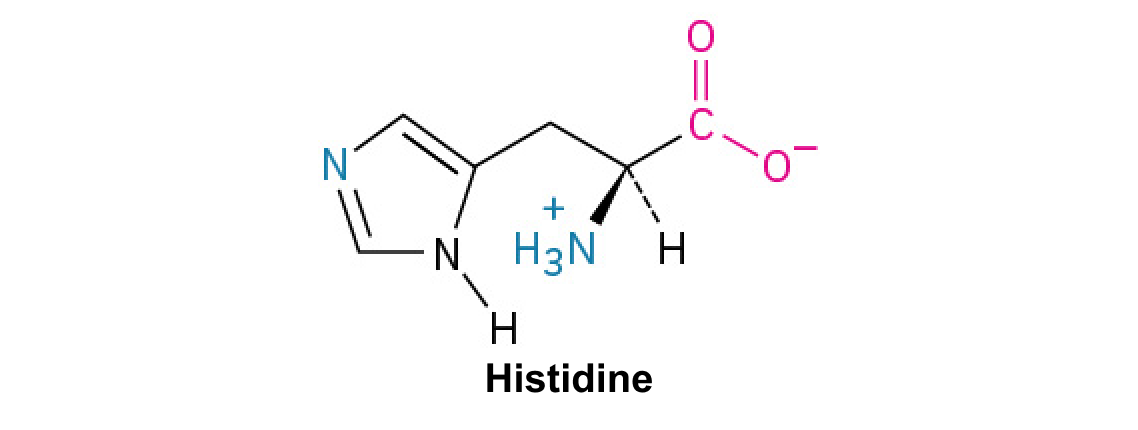
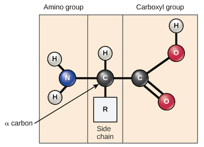
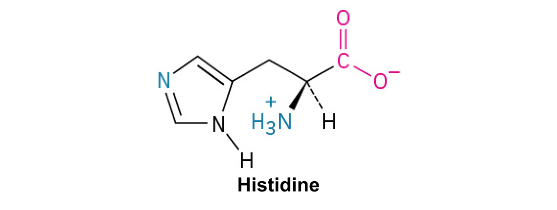
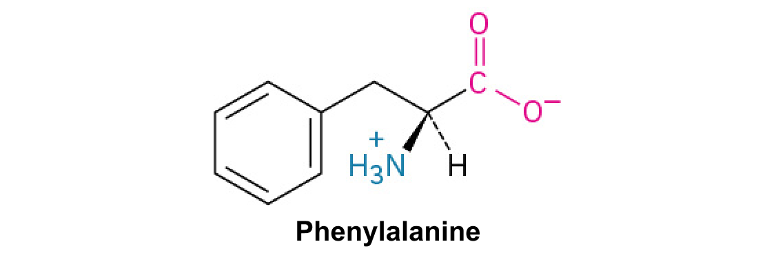
A nitrogen-containing functional group. A free amino acid’s amino group is typically protonated (NH₃⁺) near physiological pH; proline’s ring nitrogen is an exception to this formula.
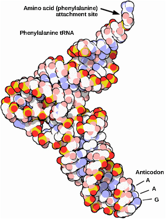
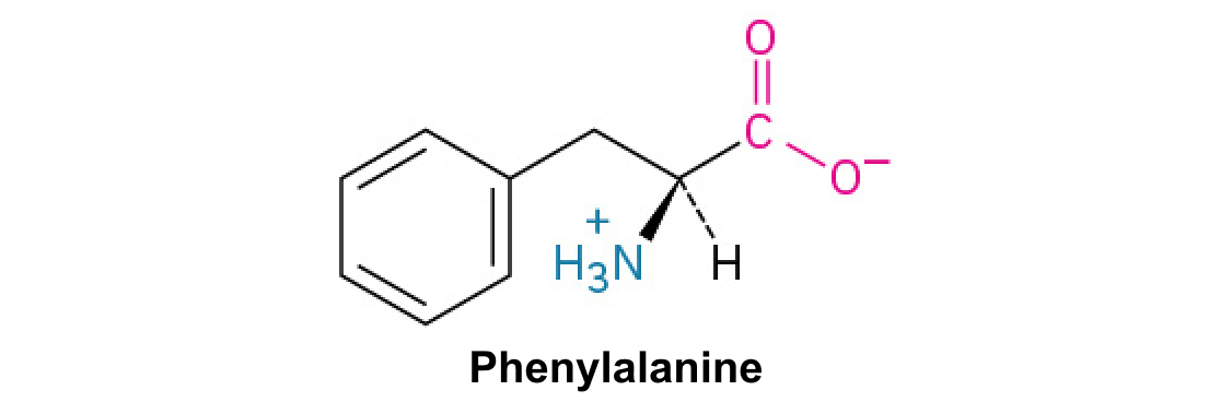
Figure 15.14 This is a space-filling model of a tRNA molecule that adds the amino acid phenylalanine to a growing polypeptide chain. The anticodon AAG binds the Codon UUC on the mRNA. The amino acid phenylalanine is attached to the other end of the tRNA.
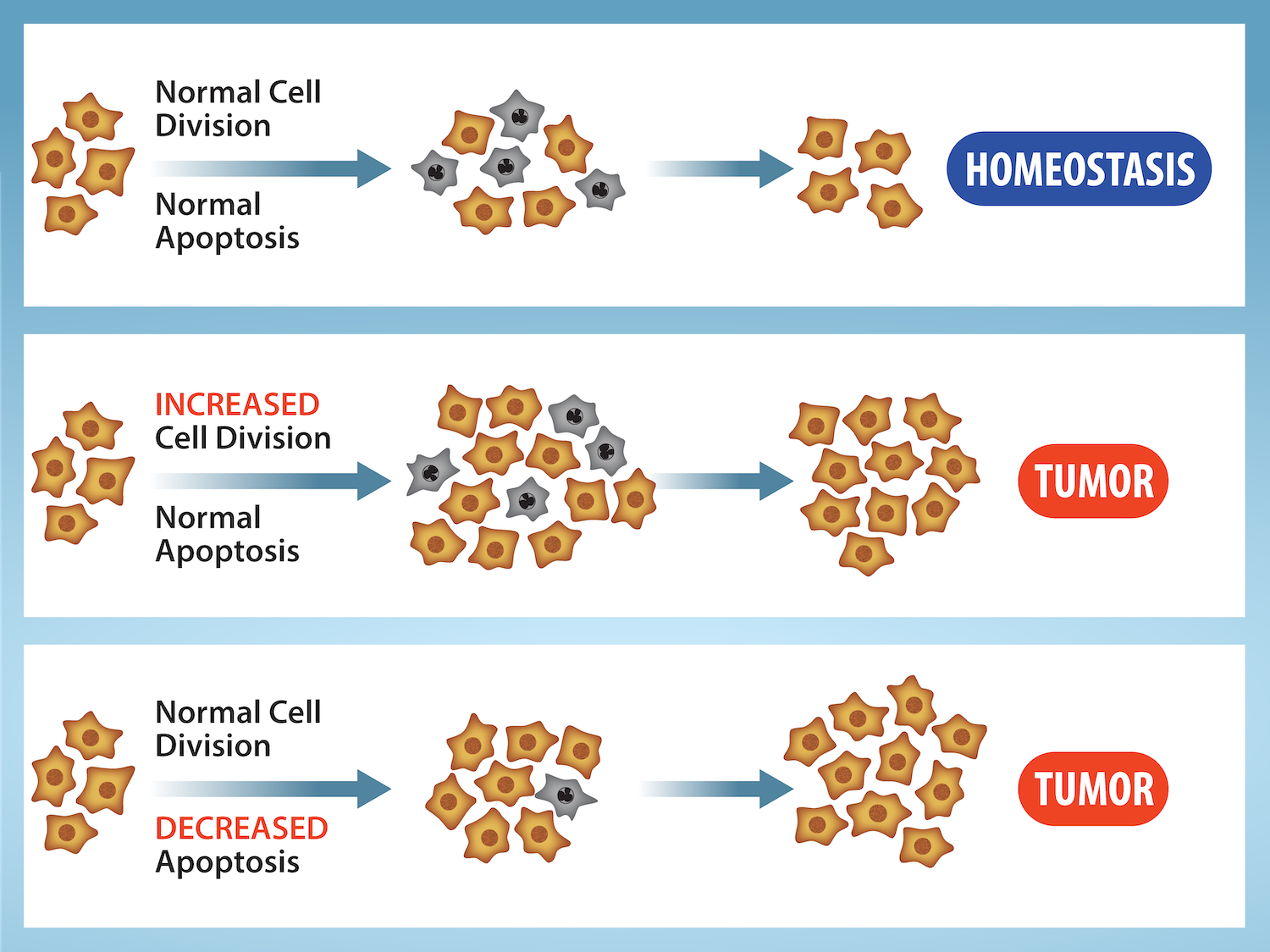
Figure 10.15 Cell Division and Apoptosis. In an adult organism, normal cell division is balanced by apoptosis (programmed cell death) to maintain a constant cell number in homeostasis. Either an increase in cell division or a decrease in apoptosis leads an increase in the number of cells and tumor formation. Credit: Rao, A. and Ryan, K. Department of Biology, Texas A&M University.
Rao, A. and Ryan, K. Department of Biology, Texas A&M University. Mary Ann Clark, Matthew Douglas, and Jung Choi, Biology 2e, OpenStax. · CC BY-NC-SA 4.0
· Original image ↗ · Access for free ↗
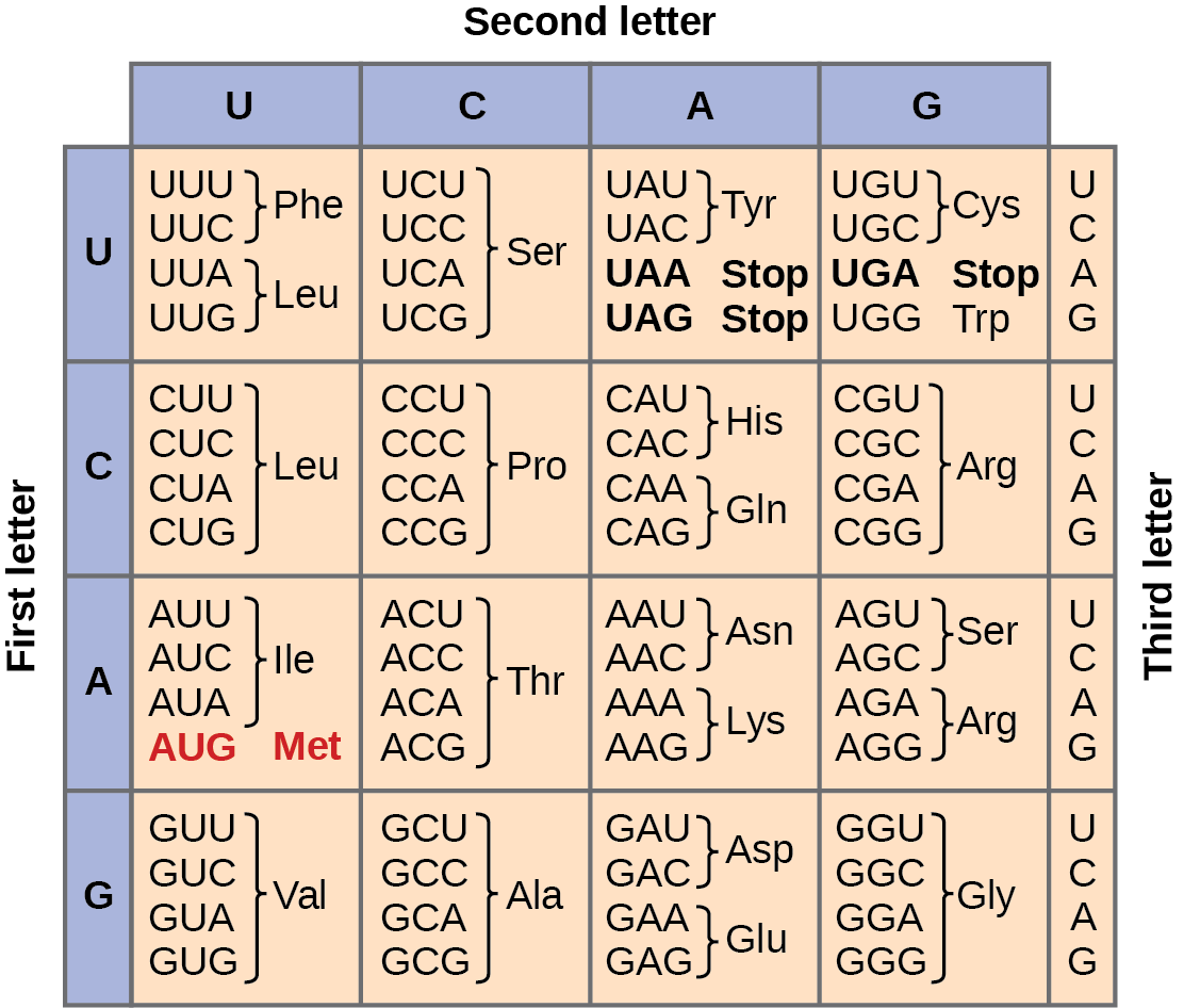
Figure 15.4 This figure shows the genetic code for translating each nucleotide triplet in mRNA into an amino acid or a termination signal in a protein. (credit: modification of work by NIH)
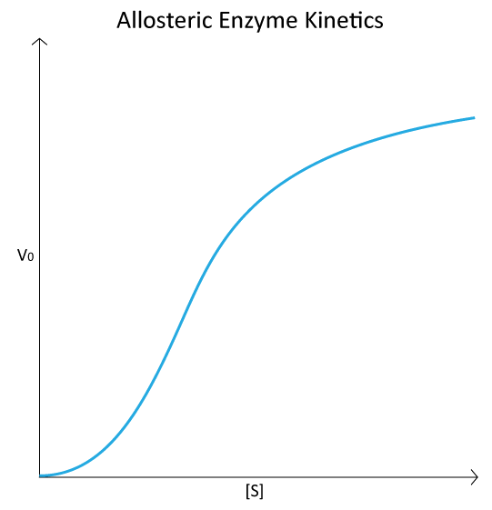
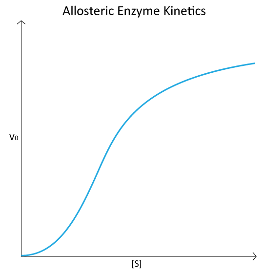
Figure 4.44 - Kinetic profile of an allosteric enzyme whose activity is controlled by a homotropic effector. Image by Aleia Kim
Kevin Ahern, Indira Rajagopal, and Taralyn Tan, Biochemistry Free For All, Oregon State University, via Biology LibreTexts. Image by Aleia Kim · CC BY-NC-SA 4.0
· Original image ↗ · Access for free ↗
An electrical property that can be positive or negative. Opposite charges attract and like charges repel; net charge is the sum of all charges on a particle.
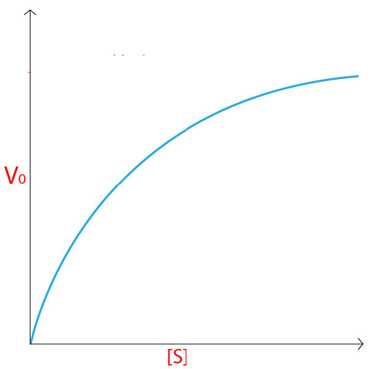
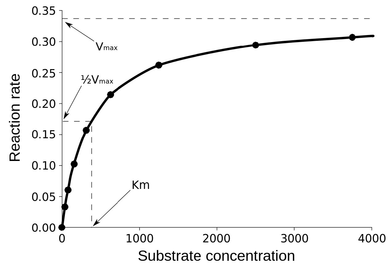
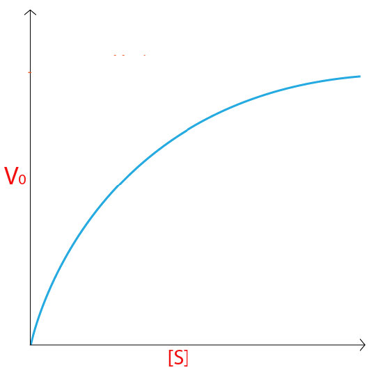
Figure 4.18 - Kinetics of an enzyme obeying Michaelis-Menten kinetics. Image by Aleia Kim
Kevin Ahern, Indira Rajagopal, and Taralyn Tan, Biochemistry Free For All, Oregon State University, via Biology LibreTexts. Image by Aleia Kim · CC BY-NC-SA 4.0
· Original image ↗ · Access for free ↗
ethnicity
Shared cultural history, ancestry, language, or affiliation.
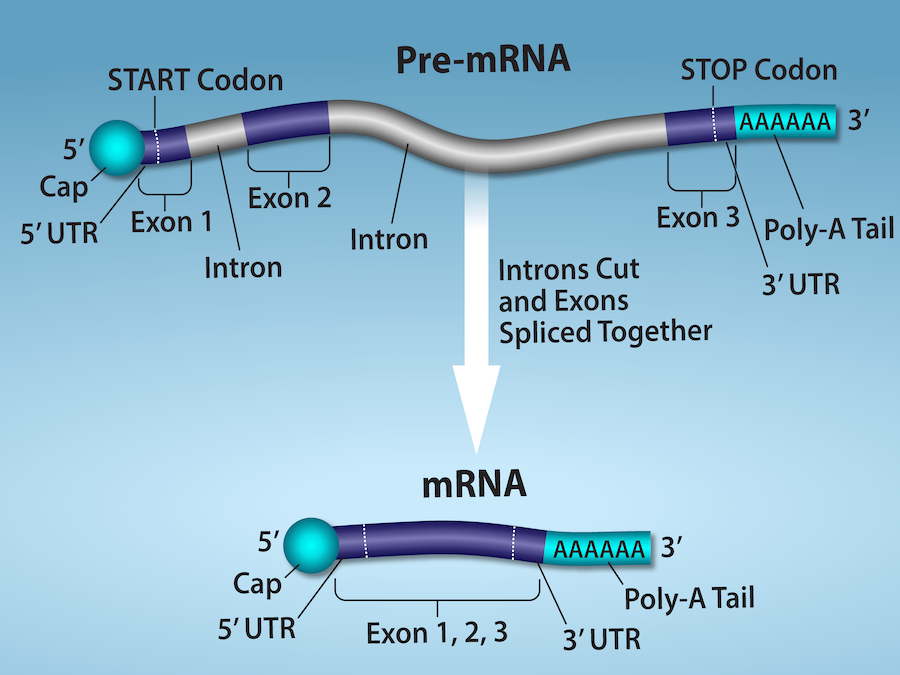
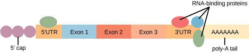
Figure 15.11 Eukaryotic pre-mRNA processing. In addition to 5’ Cap and 3’ Poly-A Tail addition, introns must be precisely removed and exons joined to generate a functional mRNA. Nucleotides upstream (towards the 5’cap) of the translation START codon are part of the 5’ untranslated region (5’ UTR). Nucleotides downstream (towards 3’end) of the STOP codon form the 3’ UTR. Both 5’ and 3’ UTRs are important for regulating translation initiation and mRNA stability. Credit: Rao, A., Ryan, K. Fletcher, S. and Tag, A. Department of Biology, Texas A&M University.
Rao, A., Ryan, K. Fletcher, S. and Tag, A. Department of Biology, Texas A&M University.; Mary Ann Clark, Matthew Douglas, and Jung Choi, Biology 2e, OpenStax. · CC BY-NC-SA 4.0
· Original image ↗ · Access for free ↗
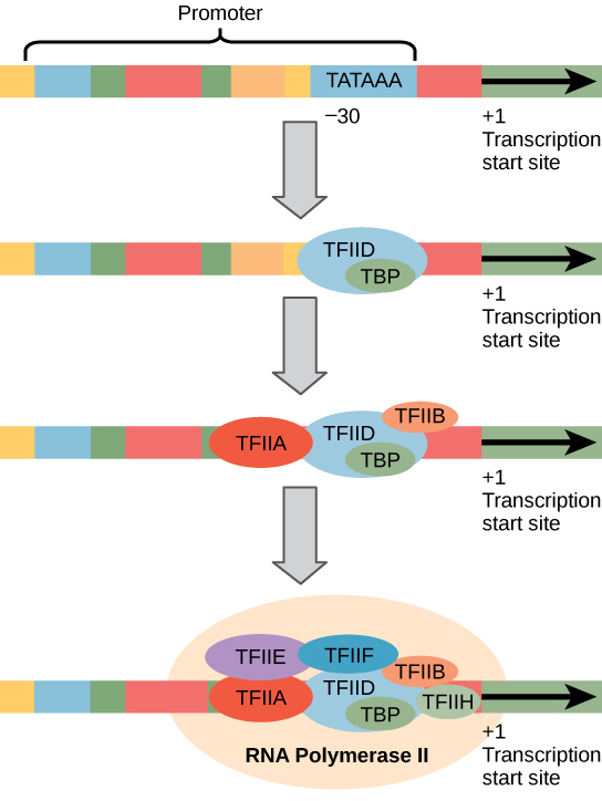
Figure 15.10 A generalized promoter of a gene transcribed by RNA polymerase II is shown. Transcription factors recognize the promoter. RNA polymerase II then binds and forms the transcription initiation complex.
Figure 16.13 RNA-binding proteins. The protein-coding region of this processed mRNA is flanked by 5' and 3' untranslated regions (UTRs). The presence of RNA-binding proteins at the 5' or 3' UTR influences the stability of the RNA molecule.
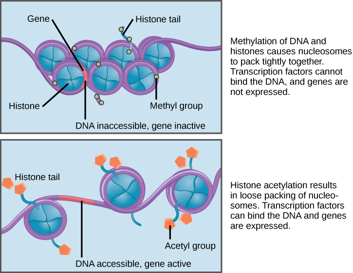
Figure 16.8 Nucleosomes can slide along DNA. When nucleosomes are spaced closely together (top), transcription factors cannot bind and gene expression is turned off. When the nucleosomes are spaced far apart (bottom), the DNA is exposed. Transcription factors can bind, allowing gene expression to occur. Modifications to the histones and DNA affect nucleosome spacing.
Figure 4.18 - Kinetics of an enzyme obeying Michaelis-Menten kinetics. Image by Aleia Kim
Kevin Ahern, Indira Rajagopal, and Taralyn Tan, Biochemistry Free For All, Oregon State University, via Biology LibreTexts. Image by Aleia Kim · CC BY-NC-SA 4.0
· Original image ↗ · Access for free ↗
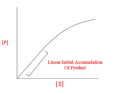
The early rate of product formation, measured before substantial substrate depletion or product accumulation, usually after the brief binding transient.
Figure 4.18 - Kinetics of an enzyme obeying Michaelis-Menten kinetics. Image by Aleia Kim
Kevin Ahern, Indira Rajagopal, and Taralyn Tan, Biochemistry Free For All, Oregon State University, via Biology LibreTexts. Image by Aleia Kim · CC BY-NC-SA 4.0
· Original image ↗ · Access for free ↗
Figure 15.11 Eukaryotic pre-mRNA processing. In addition to 5’ Cap and 3’ Poly-A Tail addition, introns must be precisely removed and exons joined to generate a functional mRNA. Nucleotides upstream (towards the 5’cap) of the translation START codon are part of the 5’ untranslated region (5’ UTR). Nucleotides downstream (towards 3’end) of the STOP codon form the 3’ UTR. Both 5’ and 3’ UTRs are important for regulating translation initiation and mRNA stability. Credit: Rao, A., Ryan, K. Fletcher, S. and Tag, A. Department of Biology, Texas A&M University.
Rao, A., Ryan, K. Fletcher, S. and Tag, A. Department of Biology, Texas A&M University.; Mary Ann Clark, Matthew Douglas, and Jung Choi, Biology 2e, OpenStax. · CC BY-NC-SA 4.0
· Original image ↗ · Access for free ↗
The exponent needed to obtain a number from a chosen fixed number. For decimal logarithms, log₁₀(100) = 2 because 10² = 100; pH uses the negative decimal logarithm of hydrogen ion activity.
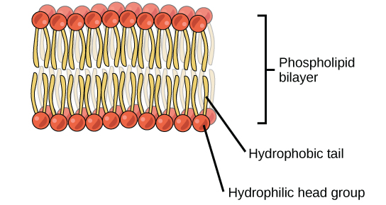
A thin boundary or sheet. Cell membranes are lipid bilayers containing proteins; blotting membranes are synthetic supports that hold proteins or nucleic acids for detection.
Figure 15.11 Eukaryotic pre-mRNA processing. In addition to 5’ Cap and 3’ Poly-A Tail addition, introns must be precisely removed and exons joined to generate a functional mRNA. Nucleotides upstream (towards the 5’cap) of the translation START codon are part of the 5’ untranslated region (5’ UTR). Nucleotides downstream (towards 3’end) of the STOP codon form the 3’ UTR. Both 5’ and 3’ UTRs are important for regulating translation initiation and mRNA stability. Credit: Rao, A., Ryan, K. Fletcher, S. and Tag, A. Department of Biology, Texas A&M University.
Rao, A., Ryan, K. Fletcher, S. and Tag, A. Department of Biology, Texas A&M University.; Mary Ann Clark, Matthew Douglas, and Jung Choi, Biology 2e, OpenStax. · CC BY-NC-SA 4.0
· Original image ↗ · Access for free ↗
Figure 4.18 - Kinetics of an enzyme obeying Michaelis-Menten kinetics. Image by Aleia Kim
Kevin Ahern, Indira Rajagopal, and Taralyn Tan, Biochemistry Free For All, Oregon State University, via Biology LibreTexts. Image by Aleia Kim · CC BY-NC-SA 4.0
· Original image ↗ · Access for free ↗
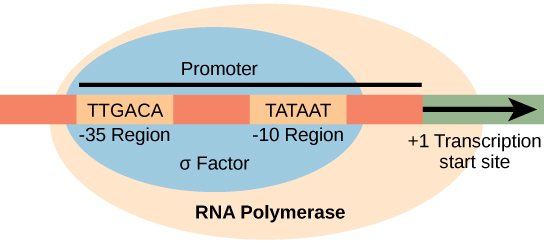
Figure 15.8 The σ subunit of prokaryotic RNA polymerase recognizes consensus sequences found in the promoter region upstream of the transcription start site. The σ subunit dissociates from the polymerase after transcription has been initiated.
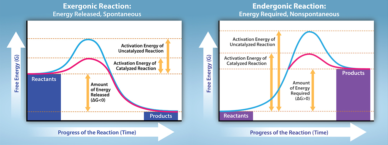
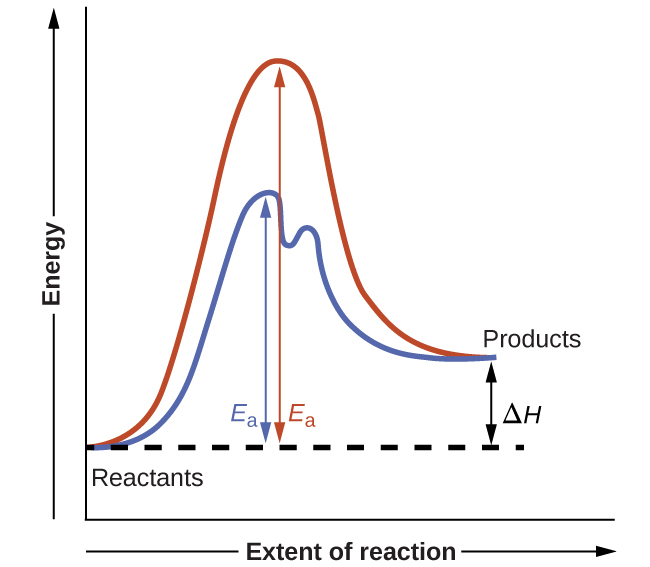
Figure 12.19 Reaction diagrams for an endothermic process in the absence (red curve) and presence (blue curve) of a catalyst. The catalyzed pathway involves a two-step mechanism (note the presence of two transition states) and an intermediate species (represented by the valley between the two transitions states).
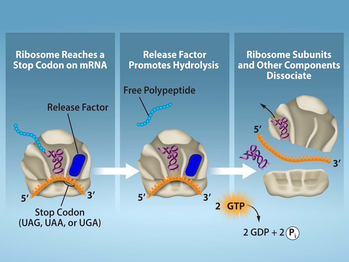
Figure 15.19 Translation Termination is Active. Translation is terminated when a STOP codon is in the A-site of the ribosome. Since there are no tRNAs corresponding to the STOP codons, the Release Factor protein enters and catalyzes the hydrolysis between the last amino acid and its tRNA. This hydrolysis releases the free carboxyl terminus (C-term) of the protein. Additional factors use the energy in GTP hydrolysis to disassemble the large and small ribosomal subunits and mRNA. Credit: Rao, A. and Ryan, K. Department of Biology, Texas A&M University.
Rao, A. and Ryan, K. Department of Biology, Texas A&M University.; Mary Ann Clark, Matthew Douglas, and Jung Choi, Biology 2e, OpenStax. · CC BY-NC-SA 4.0
· Original image ↗ · Access for free ↗
reliability
Consistency or reproducibility of a measurement under specified conditions.
In TLC, the distance traveled by a sample spot divided by the distance traveled by the solvent front, both measured from the origin. RfC, RfA, and RfB denote the values for components C, A, and B.
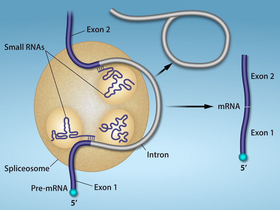
Figure 15.13 Pre-mRNA splicing involves the precise removal of introns from the primary RNA transcript. The splicing process is catalyzed by protein complexes called spliceosomes that are composed of proteins and RNA molecules called small nuclear RNAs (snRNAs). Spliceosomes recognize sequences at the 5' and 3' end of the intron. Rao, A. and Ryan, K. Department of Biology, Texas A&M University.
Rao, A. and Ryan, K. Department of Biology, Texas A&M University.; Mary Ann Clark, Matthew Douglas, and Jung Choi, Biology 2e, OpenStax. · CC BY-NC-SA 4.0
· Original image ↗ · Access for free ↗
RNA stability
Persistence of an RNA before degradation; greater stability generally means a longer lifetime or half-life under specified conditions.
Figure 16.13 RNA-binding proteins. The protein-coding region of this processed mRNA is flanked by 5' and 3' untranslated regions (UTRs). The presence of RNA-binding proteins at the 5' or 3' UTR influences the stability of the RNA molecule.
Figure 15.8 The σ subunit of prokaryotic RNA polymerase recognizes consensus sequences found in the promoter region upstream of the transcription start site. The σ subunit dissociates from the polymerase after transcription has been initiated.
Figure 4.44 - Kinetic profile of an allosteric enzyme whose activity is controlled by a homotropic effector. Image by Aleia Kim
Kevin Ahern, Indira Rajagopal, and Taralyn Tan, Biochemistry Free For All, Oregon State University, via Biology LibreTexts. Image by Aleia Kim · CC BY-NC-SA 4.0
· Original image ↗ · Access for free ↗
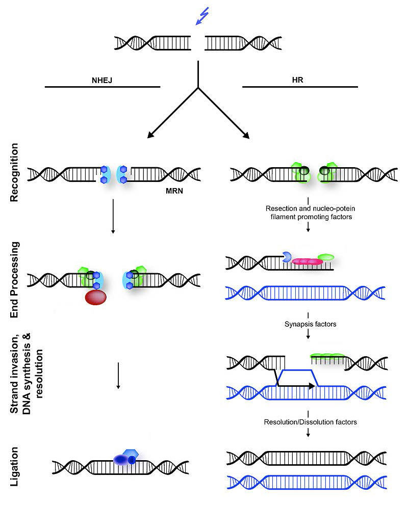
Figure 7.45 - Non-homologous end joining (left) versus homologous recombination (right) - Wikipedia
Wikipedia, as credited by Kevin Ahern, Indira Rajagopal, and Taralyn Tan, Biochemistry Free For All, Oregon State University, via Biology LibreTexts. · Source attribution
· Original image ↗ · Access for free ↗
The amount of a substance that can dissolve in a solvent under specified conditions. Soluble means able to dissolve; insoluble means only very slightly soluble in that solvent.
Figure 15.4 This figure shows the genetic code for translating each nucleotide triplet in mRNA into an amino acid or a termination signal in a protein. (credit: modification of work by NIH)
Figure 15.7 Messenger RNA is a copy of protein-coding information in the coding strand of DNA, with the substitution of U in the RNA for T in the coding sequence. However, new RNA nucleotides base pair with the nucleotides of the template strand. RNA is synthesized in its 5'-3' direction, using the enzyme RNA polymerase. As the template is read, the DNA unwinds ahead of the polymerase and then rewinds behind it.
Figure 15.14 This is a space-filling model of a tRNA molecule that adds the amino acid phenylalanine to a growing polypeptide chain. The anticodon AAG binds the Codon UUC on the mRNA. The amino acid phenylalanine is attached to the other end of the tRNA.
A fleeting, high-energy arrangement at a reaction barrier. It is an energy maximum along the reaction path, rather than a stable reaction intermediate.
Figure 12.19 Reaction diagrams for an endothermic process in the absence (red curve) and presence (blue curve) of a catalyst. The catalyzed pathway involves a two-step mechanism (note the presence of two transition states) and an intermediate species (represented by the valley between the two transitions states).
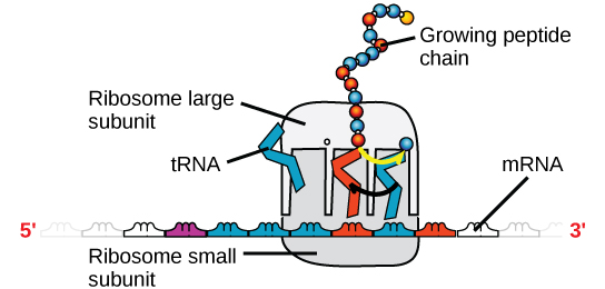
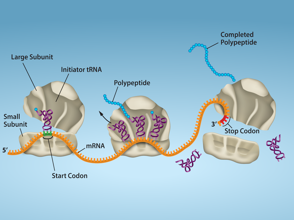
Figure 15.18 Translation begins when an initiator tRNA anticodon recognizes a start codon on mRNA bound to a small ribosomal subunit. The large ribosomal subunit joins the small subunit, and a second tRNA is recruited. As the mRNA moves relative to the ribosome, successive tRNAs move through the ribosome and the polypeptide chain is formed. Entry of a release factor into the A site terminates translation and the components dissociate.
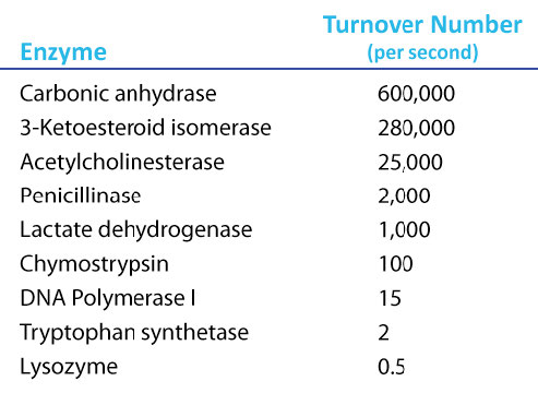
Figure 4.21 - Kcat (turnover number) values for several enzymes. Image by Aleia Kim
Kevin Ahern, Indira Rajagopal, and Taralyn Tan, Biochemistry Free For All, Oregon State University, via Biology LibreTexts. Image by Aleia Kim · CC BY-NC-SA 4.0
· Original image ↗ · Access for free ↗
Data may come from a population or from a sample. Lowercase letters like or generally are used to represent data values. Most data can be put into the following categories:
Qualitative data are the result of categorizing or describing attributes of a population. Qualitative data are also often called categorical data. Hair color, blood type, ethnic group, the car a person drives, and the street a person lives on are examples of qualitative data. Qualitative data are generally described by words or letters. For instance, hair color might be black, dark brown, light brown, blonde, gray, or red. Blood type might be AB+, O-, or B+. Researchers often prefer to use quantitative data over qualitative data because it lends itself more easily to mathematical analysis. For example, it does not make sense to find an average hair color or blood type.
Quantitative data are always numbers. Quantitative data are the result of counting or measuring attributes of a population. Amount of money, pulse rate, weight, number of people living in your town, and number of students who take statistics are examples of quantitative data. Quantitative data may be either discrete or continuous.
All data that are the result of counting are called quantitative discrete data. These data take on only certain numerical values. If you count the number of phone calls you receive for each day of the week, you might get values such as zero, one, two, or three.
Data that are not only made up of counting numbers, but that may include fractions, decimals, or irrational numbers, are called quantitative continuous data. Continuous data are often the results of measurements like lengths, weights, or times. A list of the lengths in minutes for all the phone calls that you make in a week, with numbers like 2.4, 7.5, or 11.0, would be quantitative continuous data.
The data are the number of books students carry in their backpacks. You sample five students. Two students carry three books, one student carries four books, one student carries two books, and one student carries one book. The numbers of books (three, four, two, and one) are the quantitative discrete data.
Try It
1.5
The data are the number of machines in a gym. You sample five gyms. One gym has 12 machines, one
gym has 15 machines, one gym has ten machines, one gym has 22 machines, and the other gym has 20
machines. What type of data is this?
The data are the weights of backpacks with books in them. You sample the same five students. The weights (in pounds) of their backpacks are 6.2, 7, 6.8, 9.1, 4.3. Notice that backpacks carrying three books can have different weights. Weights are quantitative continuous data.
Try It
1.6
The data are the areas of lawns in square feet. You sample five houses. The areas of the lawns are 144 sq. feet, 160 sq. feet, 190 sq. feet, 180 sq. feet, and 210 sq. feet. What type of data is this?
Example
1.7
You go to the supermarket and purchase three cans of soup (19 ounces tomato bisque, 14.1 ounces lentil, and 19 ounces Italian wedding), two packages of nuts (walnuts and peanuts), four different kinds of vegetable (broccoli, cauliflower, spinach, and carrots), and two desserts (16 ounces pistachio ice cream and 32 ounces chocolate chip cookies).
The data are the colors of backpacks. Again, you sample the same five students. One student has a red backpack, two students have black backpacks, one student has a green backpack, and one student has a gray backpack. The colors red, black, black, green, and gray are qualitative data.
Try It
1.8
The data are the colors of houses. You sample five houses. The colors of the houses are white, yellow, white, red, and white. What type of data is this?
NOTE
You may collect data as numbers and report it categorically. For example, the quiz scores for each student are recorded throughout the term. At the end of the term, the quiz scores are reported as A, B, C, D, or F.
Example
1.9
Problem
Work collaboratively to determine the correct data type (quantitative or qualitative). Indicate whether quantitative data are continuous or discrete. Hint: Data that are discrete often start with the words "the number of."
the number of pairs of shoes you own
the type of car you drive
the distance it is from your home to the nearest grocery store
Determine the correct data type (quantitative or qualitative) for the number of cars in a parking lot. Indicate whether quantitative data are continuous or discrete.
Example
1.10
Problem
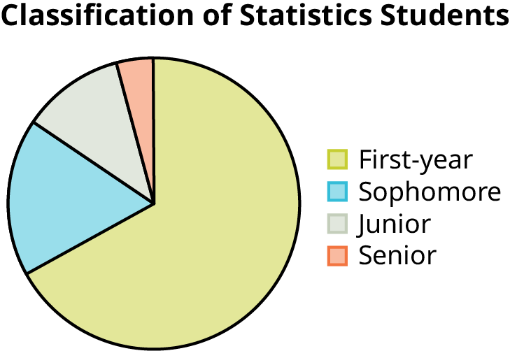
A statistics professor collects information about the classification of her students as first-year students, sophomores, juniors, or seniors. The data she collects are summarized in the pie chart Figure 1.3. What type of data does this graph show?
Figure 1.3 — 1.2 Data, Sampling, and Variation in Data and Sampling
This pie chart shows the students in each year, which is qualitative (or categorical) data.
Try It
1.10
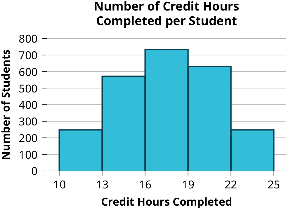
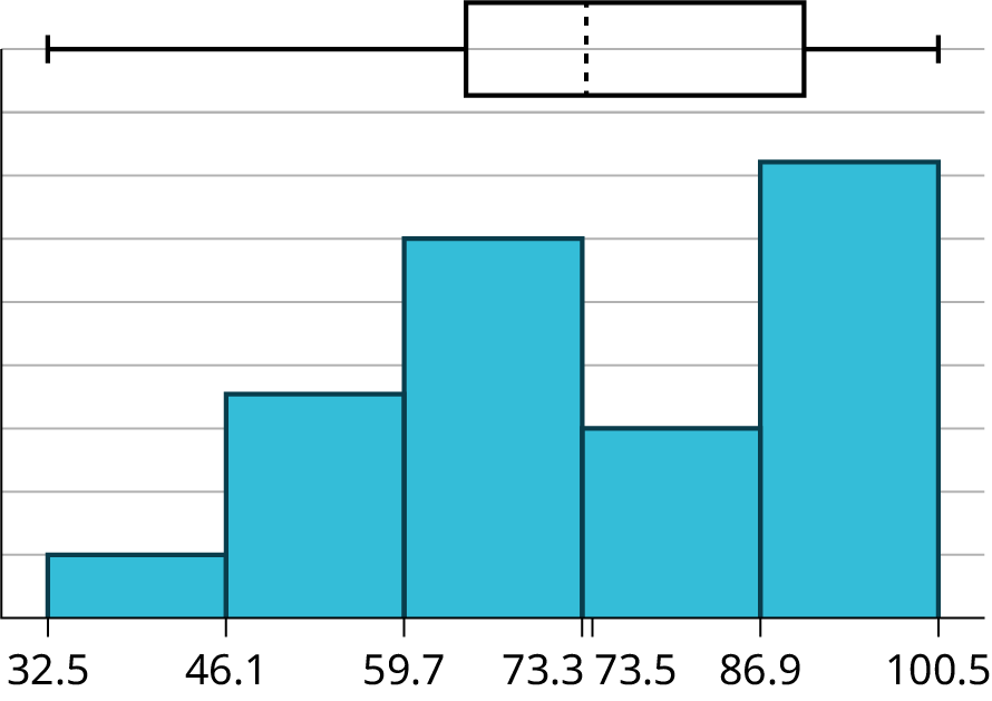
The registrar at State University keeps records of the number of credit hours students complete each semester. The data collected are summarized in the histogram. The class boundaries are 10 to less than 13, 13 to less than 16, 16 to less than 19, 19 to less than 22, and 22 to less than 25.
Figure 1.4 — 1.2 Data, Sampling, and Variation in Data and Sampling
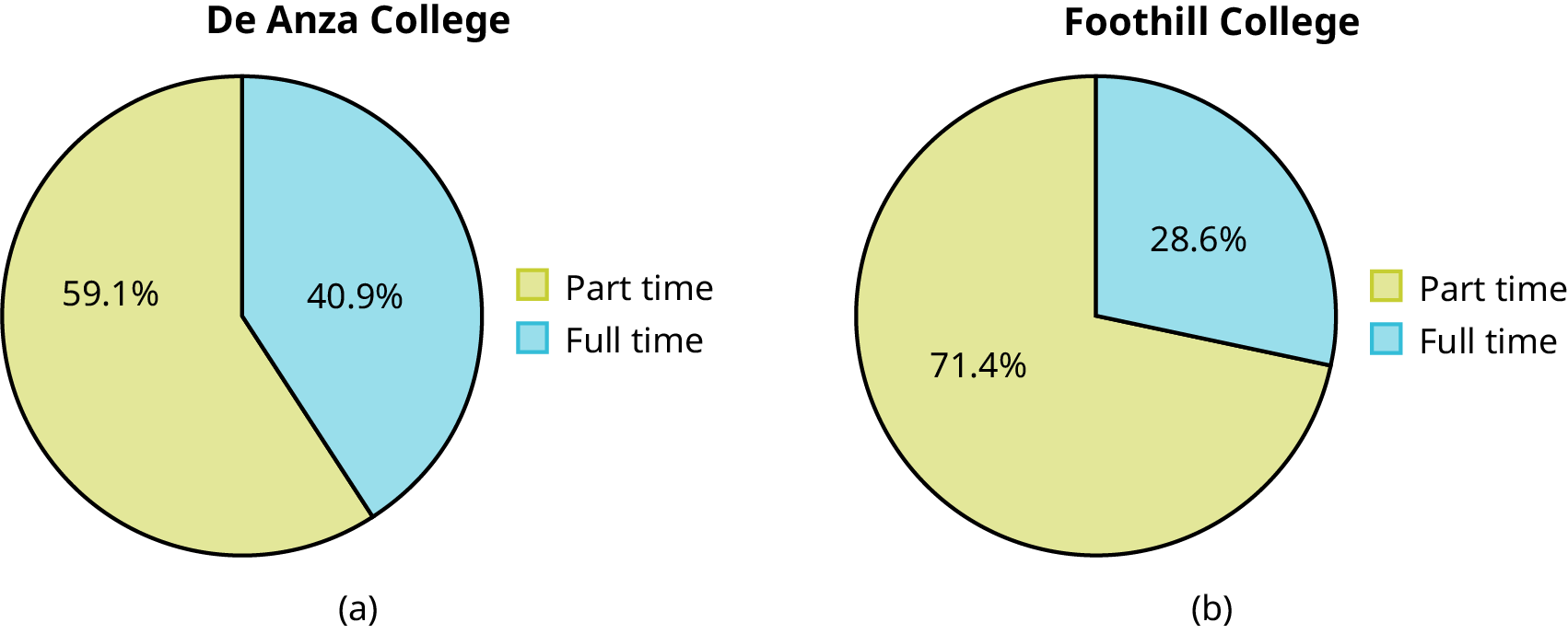
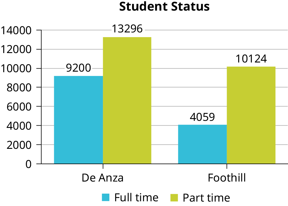
Below are tables comparing the number of part-time and full-time students at De Anza College and Foothill College enrolled for the most recent spring quarter. The tables display counts (frequencies) and percentages or proportions (relative frequencies). The percent columns make comparing the same categories in the colleges easier. Displaying percentages along with the numbers is often helpful, but it is particularly important when comparing sets of data that do not have the same totals, such as the total enrollments for both colleges in this example. Notice how much larger the percentage for part-time students at Foothill College is compared to De Anza College.
De Anza College
Foothill College
Number
Percent
Number
Percent
Full-time
9,200
40.9%
Full-time
4,059
28.6%
Part-time
13,296
59.1%
Part-time
10,124
71.4%
Total
22,496
100%
Total
14,183
100%
Table
1.3
Most Recent Spring Quarter
Tables are a good way of organizing and displaying data. But graphs can be even more helpful in understanding the data. There are no strict rules concerning which graphs to use. Two graphs that are used to display qualitative data are pie charts and bar graphs.
In a pie chart, categories of data are represented by wedges in a circle and are proportional in size to the percent of individuals in each category.
In a bar graph, the length of the bar for each category is proportional to the number or percent of individuals in each category. Bars may be vertical or horizontal.
A Pareto chart consists of bars that are sorted into order by category size (largest to smallest).
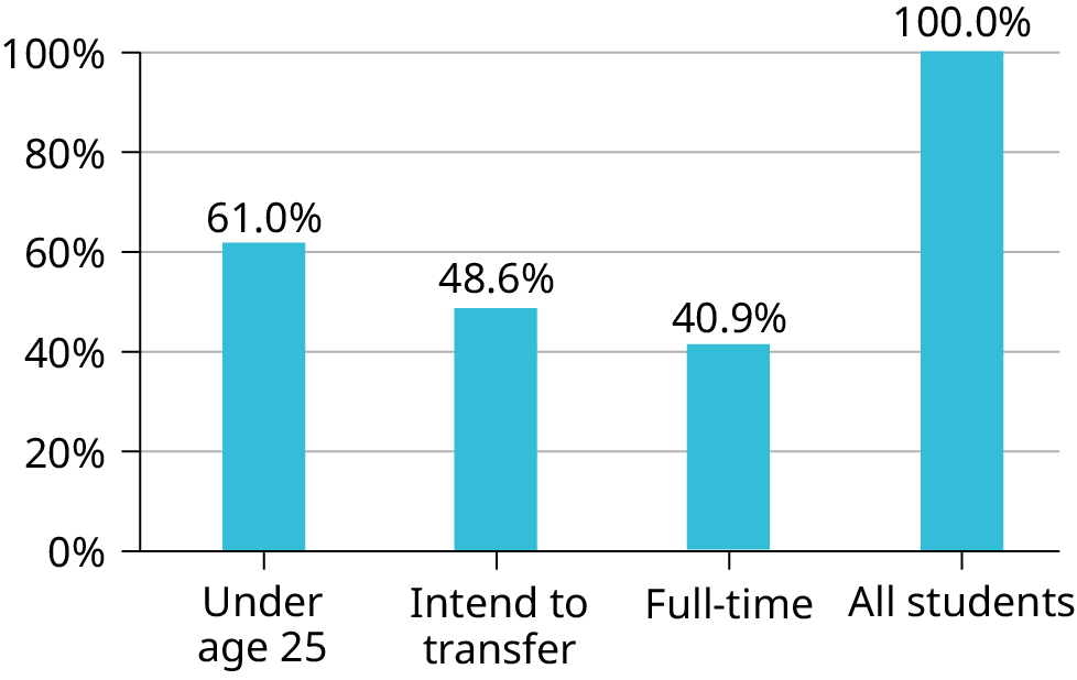
Look at Figure 1.5 and Figure 1.6 and determine which graph (pie or bar) you think displays the comparisons better.
It is a good idea to look at a variety of graphs to see which is the most helpful in displaying the data. We might make different choices of what we think is the “best” graph depending on the data and the context. Our choice also depends on what we are using the data for.
Figure 1.5 — 1.2 Data, Sampling, and Variation in Data and Sampling
Sometimes percentages add up to be more than 100% (or less than 100%). In the graph, the percentages add to more than 100% because students can be in more than one category. A bar graph is appropriate to compare the relative size of the categories. A pie chart cannot be used. It also could not be used if the percentages added to less than 100%.
Characteristic/Category
Percent
Full-Time Students
40.9%
Students who intend to transfer to a 4-year educational institution
48.6%
Students under age 25
61.0%
TOTAL
150.5%
Table
1.4
De Anza College Most Recent Spring Quarter
Figure 1.7 — 1.2 Data, Sampling, and Variation in Data and Sampling
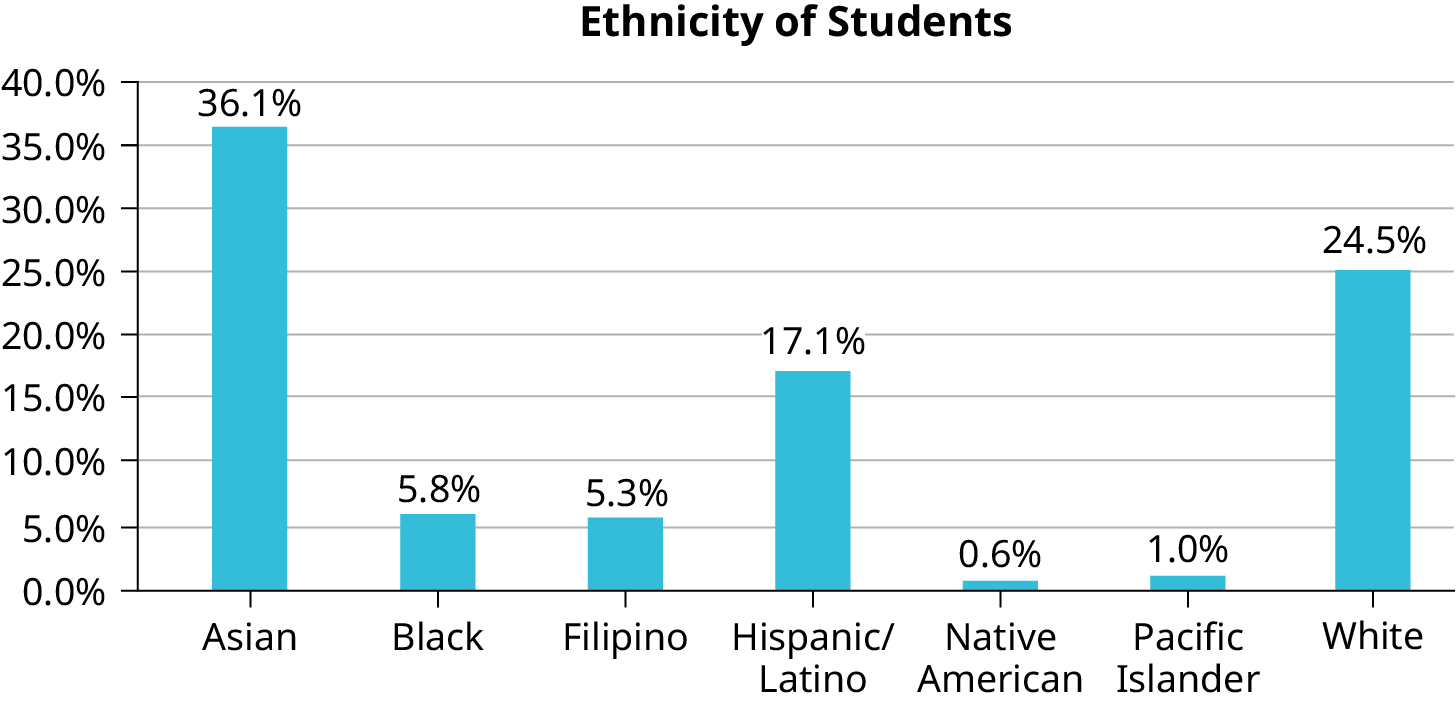
The table displays Ethnicity of Students but is missing the "Other/Unknown" category. This category contains people who did not feel they fit into any of the ethnicity categories or declined to respond. Notice that the frequencies do not add up to the total number of students. In this situation, create a bar graph and not a pie chart.
Frequency
Percent
Asian
8,794
36.1%
Black
1,412
5.8%
Filipino
1,298
5.3%
Hispanic/Latino
4,180
17.1%
Native American
146
0.6%
Pacific Islander
236
1.0%
White
5,978
24.5%
TOTAL
22,044 out of 24,382
90.4% out of 100%
Table
1.5
Ethnicity of Students at De Anza College in the Most Recent Fall Term
Figure 1.8 — 1.2 Data, Sampling, and Variation in Data and Sampling
The following graph is the same as the previous graph but the “Other/Unknown” percent (9.6%) has been included. The “Other/Unknown” category is large compared to some of the other categories (Native American, 0.6%, Pacific Islander 1.0%). This is important to know when we think about what the data are telling us.
This particular bar graph in Figure 1.9 can be difficult to understand visually. The graph in Figure 1.10 is a Pareto chart. The Pareto chart has the bars sorted from largest to smallest and is easier to read and interpret.
Figure 1.9 — 1.2 Data, Sampling, and Variation in Data and Sampling
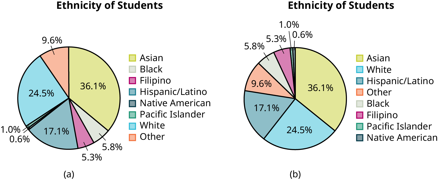
The following pie charts have the “Other/Unknown” category included (since the percentages must add to 100%). The chart in Figure 1.11(b) is organized by the size of each wedge, which makes it a more visually informative graph than the unsorted, alphabetical graph in Figure 1.11(a).
Figure 1.11 — 1.2 Data, Sampling, and Variation in Data and Sampling
Gathering information about an entire population often costs too much or is virtually impossible. Instead, we use a sample of the population. A sample should have the same characteristics as the population it is representing. Most statisticians use various methods of random sampling in an attempt to achieve this goal. This section will describe a few of the most common methods. There are several different methods of random sampling. In each form of random sampling, each member of a population initially has an equal chance of being selected for the sample. Each method has pros and cons. The easiest method to describe is called a simple random sample. Any group of n individuals is equally likely to be chosen as any other group of n individuals if the simple random sampling technique is used. In other words, each sample of the same size has an equal chance of being selected. For example, suppose Lisa wants to form a four-person study group (herself and three other people) from her pre-calculus class, which has 31 members not including Lisa. To choose a simple random sample of size three from the other members of her class, Lisa could put all 31 names in a hat, shake the hat, close her eyes, and pick out three names. A more technological way is for Lisa to first list the last names of the members of her class together with a two-digit number, as in Table 1.6:
ID
Name
ID
Name
ID
Name
00
Anselmo
11
King
21
Roquero
01
Bautista
12
Legeny
22
Roth
02
Bayani
13
Lundquist
23
Rowell
03
Cheng
14
Macierz
24
Salangsang
04
Cuarismo
15
Motogawa
25
Slade
05
Cuningham
16
Okimoto
26
Stratcher
06
Fontecha
17
Patel
27
Tallai
07
Hong
18
Price
28
Tran
08
Hoobler
19
Quizon
29
Wai
09
Jiao
20
Reyes
30
Wood
10
Khan
Table
1.6
Class Roster
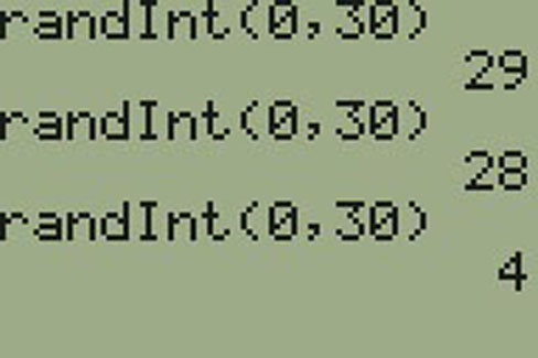
Lisa can use a table of random numbers (found in many statistics books and mathematical handbooks), a calculator, or a computer to generate random numbers. For this example, suppose Lisa chooses to generate random numbers from a calculator. The numbers generated are as follows:
Lisa reads two-digit groups until she has chosen three class members (that is, she reads 0.94360 as the
groups 94, 43, 36, 60). Each random number may only contribute one class member. If she needed to, Lisa
could have generated more random numbers.
The random numbers 0.94360 and 0.99832 do not contain appropriate two digit numbers. However the third random number, 0.14669, contains 14 (the fourth random number also contains 14), the fifth random number contains 05, and the seventh random number contains 04. The two-digit number 14 corresponds to Macierz, 05 corresponds to Cuningham, and 04 corresponds to Cuarismo. Besides herself, Lisa’s group will consist of Marcierz, Cuningham, and Cuarismo.
Using the TI-83, 83+, 84, 84+ Calculator
To generate random numbers:
Press MATH.
Arrow over to PRB.
Press 5:randInt(. Enter 0, 30).
Press ENTER for the first random number.
Press ENTER two more times for the other 2 random numbers. If there is a repeat press ENTER again.
Note: randInt(0, 30, 3) will generate 3 random numbers.
Figure 1.12 — 1.2 Data, Sampling, and Variation in Data and Sampling
Besides simple random sampling, there are other forms of sampling that involve a chance process for getting the sample. Other well-known random sampling methods are the stratified sample, the cluster sample, and the systematic sample.
To choose a stratified sample, divide the population into groups called strata and then take a proportionate number from each stratum. For example, you could stratify (group) your college population by department and then choose a proportionate simple random sample from each stratum (each department) to get a stratified random sample. To choose a simple random sample from each department, number each member of the first department, number each member of the second department, and do the same for the remaining departments. Then use simple random sampling to choose proportionate numbers from the first department and do the same for each of the remaining departments. Those numbers picked from the first department, picked from the second department, and so on represent the members who make up the stratified sample.
To choose a cluster sample, divide the population into clusters (groups) and then randomly select some of the clusters. All the members from these clusters are in the cluster sample. For example, if you randomly sample four departments from your college population, the four departments make up the cluster sample. Divide your college faculty by department. The departments are the clusters. Number each department, and then choose four different numbers using simple random sampling. All members of the four departments with those numbers are the cluster sample.
To choose a systematic sample, randomly select a starting point and take every nth piece of data from a listing of the population. For example, suppose you have to do a phone survey. Your phone book contains 20,000 residence listings. You must choose 400 names for the sample. Number the population 1–20,000 and then use a simple random sample to pick a number that represents the first name in the sample. Then choose every fiftieth name thereafter until you have a total of 400 names (you might have to go back to the beginning of your phone list). Systematic sampling is frequently chosen because it is a simple method.
A type of sampling that is non-random is convenience sampling. Convenience sampling involves using results that are readily available. For example, a computer software store conducts a marketing study by interviewing potential customers who happen to be in the store browsing through the available software. The results of convenience sampling may be very good in some cases and highly biased (favor certain outcomes) in others.
Sampling data should be done very carefully. Collecting data carelessly can have devastating results. Surveys mailed to households and then returned may be very biased (they may favor a certain group). It is better for the person conducting the survey to select the sample respondents.
Sampling with replacement is truly random sampling. That is, once a member is picked, that member goes back into the population and thus may be chosen more than once. However for practical reasons, in most populations, simple random sampling without replacement is done. Surveys are typically done without replacement. That is, a member of the population may be chosen only once. Most samples are taken from large populations and the sample tends to be small in comparison to the population. Since this is the case, sampling without replacement is approximately the same as sampling with replacement because the chance of picking the same individual more than once with replacement is very low.
Sampling without replacement instead of sampling with replacement becomes a mathematical issue only when the population is small.
When you analyze data, it is important to be aware of sampling errors and nonsampling errors. The actual process of sampling causes sampling errors. For example, the sample may not be large enough. Factors not related to the sampling process cause nonsampling errors. A defective counting device can cause a nonsampling error.
In reality, a sample will never be exactly representative of the population so there will always be some sampling error. As a rule, the larger the sample, the smaller the sampling error.
In statistics, a sampling bias is created when a sample is collected from a population and some members of the population are not as likely to be chosen as others (remember, each member of the population should have an equally likely chance of being chosen). When a sampling bias happens, there can be incorrect conclusions drawn about the population that is being studied.
Critical Evaluation
We need to evaluate the statistical studies we read about critically and analyze them before accepting the results of the studies. Common problems to be aware of include
Problems with samples: A sample must be representative of the population. A sample that is not representative of the population is biased. Biased samples that are not representative of the population give results that are inaccurate and not valid.
Self-selected samples: Responses only by people who choose to respond, such as call-in
surveys, are often unreliable.
Sample size issues: Samples that are too small may be unreliable. Larger samples are better, if possible. In some situations, having small samples is unavoidable and can still be used to draw conclusions. Examples: crash testing cars or medical testing for rare conditions
Undue influence: collecting data or asking questions in a way that influences the response
Non-response or refusal of subject to participate: The collected responses may no longer be representative of the population. Often, people with strong positive or negative opinions may answer surveys, which can affect the results.
Causality: A relationship between two variables does not mean that one causes the other to occur. They may be related (correlated) because of their relationship through a different variable.
Self-funded or self-interest studies: A study performed by a person or organization in order to support their claim. Is the study impartial? Read the study carefully to evaluate the work. Do not automatically assume that the study is good, but do not automatically assume the study is bad either. Evaluate it on its merits and the work done.
Misleading use of data: improperly displayed graphs, incomplete data, or lack of context
Confounding: When the effects of multiple factors on a response cannot be separated. Confounding makes it difficult or impossible to draw valid conclusions about the effect of each factor.
Collaborative Exercise
As a class, determine whether or not the following samples are representative. If they are not, discuss the reasons.
To find the average GPA of all students in a university, use all honor students at the university as the sample.
To find out the most popular cereal among young people under the age of ten, stand outside a large supermarket for three hours and speak to every twentieth child under age ten who enters the supermarket.
To find the average annual income of all adults in the United States, sample U.S. Representatives. Create a cluster sample by considering each state as a stratum (group). By using simple random sampling, select states to be part of the cluster. Then survey every U.S. Representative in the cluster.
To determine the proportion of people taking public transportation to work, survey 20 people in New York City. Conduct the survey by sitting in Central Park on a bench and interviewing every person who sits next to you.
To determine the average cost of a two-day stay in a hospital in Massachusetts, survey 100 hospitals across the state using simple random sampling.
Example
1.11
Problem
A study is done to determine the average tuition that San Jose State undergraduate students pay per semester. Each student in the following samples is asked how much tuition they paid for the Fall semester. What is the type of sampling in each case?
A sample of 100 undergraduate San Jose State students is taken by organizing the students’ names by classification (first-year, sophomore, junior, or senior), and then selecting 25 students from each.
A random number generator is used to select a student from the alphabetical listing of all undergraduate students in the Fall semester. Starting with that student, every 50th student is chosen until 75 students are included in the sample.
A completely random method is used to select 75 students. Each undergraduate student in the fall semester has the same probability of being chosen at any stage of the sampling process.
The first-year, sophomore, junior, and senior years are numbered one, two, three, and four, respectively. A random number generator is used to pick two of those years. All students in those two years are in the sample.
An administrative assistant is asked to stand in front of the library one Wednesday and to ask the first 100 undergraduate students he encounters what they paid for tuition the Fall semester. Those 100 students are the sample.
a. stratified; b. systematic; c. simple random; d. cluster; e. convenience
Try It
1.11
You are going to use the random number generator to generate different types of samples from the data.
This table displays six sets of quiz scores (each quiz counts 10 points) for an elementary statistics class.
#1
#2
#3
#4
#5
#6
5
7
10
9
8
3
10
5
9
8
7
6
9
10
8
6
7
9
9
10
10
9
8
9
7
8
9
5
7
4
9
9
9
10
8
7
7
7
10
9
8
8
8
8
9
10
8
8
9
7
8
7
7
8
8
8
10
9
8
7
Table
1.7
Instructions: Use the Random Number Generator to pick samples.
Create a stratified sample by column. Pick three quiz scores randomly from each column.
Number each row one through ten.
On your calculator, press Math and arrow over to PRB.
For column 1, Press 5:randInt( and enter 1,10). Press ENTER. Record the number. Press ENTER 2 more times (even the repeats). Record these numbers. Record the three quiz scores in column one that correspond to these three numbers.
Repeat for columns two through six.
These 18 quiz scores are a stratified sample.
Create a cluster sample by picking two of the columns. Use the column numbers: one through six.
Press MATH and arrow over to PRB.
Press 5:randInt( and enter 1,6). Press ENTER. Record the number. Press ENTER and record that number.
The two numbers are for two of the columns.
The quiz scores (20 of them) in these 2 columns are the cluster sample.
Create a simple random sample of 15 quiz scores.
Use the numbering one through 60.
Press MATH. Arrow over to PRB. Press 5:randInt( and enter 1, 60).
Press ENTER 15 times and record the numbers.
Record the quiz scores that correspond to these numbers.
These 15 quiz scores are the random sample.
Create a systematic sample of 12 quiz scores.
Use the numbering one through 60.
Press MATH. Arrow over to PRB. Press 5:randInt( and enter 1, 60).
Press ENTER. Record the number and the first quiz score. From that number, count ten quiz scores and record that quiz score. Keep counting ten quiz scores and recording the quiz score until you have a sample of 12 quiz scores. You may wrap around (go back to the beginning).
Example
1.12
Problem
Determine the type of sampling used (simple random, stratified, systematic, cluster, or convenience).
A soccer coach selects six players from a group of boys aged eight to ten, seven players from a group of boys aged 11 to 12, and three players from a group of boys aged 13 to 14 to form a recreational soccer team.
A pollster interviews all human resource personnel in five different high tech companies.
A high school educational researcher interviews 50 public high school teachers and 50 private high school teachers.
A medical researcher interviews every third cancer patient from a list of cancer patients at a local hospital.
A high school counselor uses a computer to generate 50 random numbers and then picks students whose names correspond to the numbers.
A student interviews classmates in their algebra class to determine how many pairs of jeans a student owns, on the average.
a. stratified; b. cluster; c. stratified; d. systematic; e. simple random; f.convenience
Try It
1.12
Determine the type of sampling used (simple random, stratified, systematic, cluster, or convenience).
A high school principal polls 50 first-year students, 50 sophomores, 50 juniors, and 50 seniors regarding policy changes for after school activities.
If we were to examine two samples representing the same population, even if we used random sampling methods for the samples, they would not be exactly the same. Just as there is variation in data, there is variation in samples. As you become accustomed to sampling, the variability will begin to seem natural.
NOTE
In Confidence Intervals of the text, sample size formulas are provided which will determine sample sizes when sampling from a population. The sample size will be a function of the desired precision and not a function of the population size. It may be somewhat counterintuitive that the sample size does not depend on the population size. However, this implies that a sample size of 1,000 can be adequate to represent a population of 100,000 versus 1,000,000 given that the same level of precision is desired. When working in Confidence Intervals with sample size formulas, the student will notice that population size is not a factor in determining the sample size.
Example
1.13
Suppose ABC College has 10,000 part-time students (the population). We are interested in the average amount of money a part-time student spends on books in the fall term. Asking all 10,000 students is an almost impossible task.
Suppose we take two different samples.
First, we use convenience sampling and survey ten students from a first term organic chemistry class. Many of these students are taking first term calculus in addition to the organic chemistry class. The amount of money they spend on books is as follows:
The second sample is taken using a list of senior citizens who take P.E. classes and taking every fifth senior citizen on the list, for a total of ten senior citizens. They spend:
$50;
$40;
$36;
$15;
$50;
$100;
$40;
$53;
$22;
$22
It is unlikely that any student is in both samples.
Problem
a. Do you think that either of these samples is representative of (or is characteristic of) the entire 10,000 part-time student population?
a. No. The first sample probably consists of science-oriented students. Besides the chemistry course, some of them are also taking first-term calculus. Books for these classes tend to be expensive. Most of these students are, more than likely, paying more than the average part-time student for their books. The second sample is a group of senior citizens who are, more than likely, taking courses for health and interest. The amount of money they spend on books is probably much less than the average part-time student. Both samples are biased. Also, in both cases, not all students have a chance to be in either sample.
Problem
b. Since these samples are not representative of the entire population, is it wise to use the results to describe the entire population?
b. No. For these samples, each member of the population did not have an equally likely chance of being chosen.
Now, suppose we take a third sample. We choose ten different part-time students from the disciplines of chemistry, math, English, psychology, sociology, history, nursing, physical education, art, and early childhood development. (We assume that these are the only disciplines in which part-time students at ABC College are enrolled and that an equal number of part-time students are enrolled in each of the disciplines.) Each student is chosen using simple random sampling. Using a calculator, random numbers are generated and a student from a particular discipline is selected if they have a corresponding number. The students spend the following amounts:
c. The sample is unbiased, but a larger sample would be recommended to increase the likelihood that the sample will be close to representative of the population. However, for a biased sampling technique, even a large sample runs the risk of not being representative of the population.
Students often ask if it is "good enough" to take a sample, instead of surveying the entire population. If the survey is done well, the answer is yes.
Try It
1.13
A local radio station has a fan base of 20,000 listeners. The station wants to know if its audience would prefer more music or more talk shows. Asking all 20,000 listeners is an almost impossible task.
The station uses convenience sampling and surveys the first 200 people they meet at one of the station’s music concert events. 24 people said they’d prefer more talk shows, and 176 people said they’d prefer more music.
Do you think that this sample is representative of (or is characteristic of) the entire 20,000 listener population?
Variation in Data
Variation is present in any set of data. For example, 16-ounce cans of beverage may contain more or less than 16 ounces of liquid. In one study, eight 16-ounce cans were measured and produced the following amount (in ounces) of beverage:
15.8;
16.1;
15.2;
14.8;
15.8;
15.9;
16.0;
15.5
Measurements of the amount of beverage in a 16-ounce can may vary because different people make the measurements or because the exact amount, 16 ounces of liquid, was not put into the cans. Manufacturers regularly run tests to determine if the amount of beverage in a 16-ounce can falls within the desired range.
Be aware that as you take data, your data may vary somewhat from the data someone else is taking for the same purpose. This is completely natural. However, if two or more of you are taking the same data and get very different results, it is time for you and the others to reevaluate your data-taking methods and your accuracy.
Variation in Samples
It was mentioned previously that two or more samples from the same population, taken randomly, and having close to the same characteristics of the population will likely be different from each other. Suppose Doreen and Jung both decide to study the average amount of time students at their college sleep each night. Doreen and Jung each take samples of 500 students. Doreen uses systematic sampling and Jung uses cluster sampling. Doreen's sample will be different from Jung's sample. Even if Doreen and Jung used the same sampling method, in all likelihood their samples would be different. Neither would be wrong, however.
Think about what contributes to making Doreen’s and Jung’s samples different.
If Doreen and Jung took larger samples (i.e. the number of data values is increased), their sample results (the average amount of time a student sleeps) might be closer to the actual population average. But still, their samples would be, in all likelihood, different from each other. This variability in samples cannot be stressed enough.
Size of a Sample
The size of a sample (often called the number of observations) is important. The examples you have seen in this book so far have been small. Samples of only a few hundred observations, or even smaller, are sufficient for many purposes. In polling, samples that are from 1,200 to 1,500 observations are considered large enough and good enough if the survey is random and is well done. You will learn why when you study confidence intervals.
Be aware that many large samples are biased. For example, call-in surveys are invariably biased, because people choose to respond or not.
Collaborative Exercise
Divide into groups of two, three, or four. Your instructor will give each group one six-sided die. Try this experiment twice. Roll one fair die (six-sided) 20 times. Record the number of ones, twos, threes, fours, fives, and sixes you get in Table 1.8 and Table 1.9 (“frequency” is the number of times a particular face of the die occurs):
Face on Die
Frequency
1
2
3
4
5
6
Table
1.8
First Experiment (20 rolls)
Face on Die
Frequency
1
2
3
4
5
6
Table
1.9
Second Experiment (20 rolls)
Did the two experiments have the same results? Probably not. If you did the experiment a third time, do you expect the results to be identical to the first or second experiment? Why or why not?
Which experiment had the correct results? They both did. The job of the statistician is to see through the variability and draw appropriate conclusions.
9.4 Rare Events, the Sample, Decision and Conclusion
Establishing the type of distribution, sample size, and known or unknown standard deviation can help you figure out how to go about a hypothesis test. However, there are several other factors you should consider when working out a hypothesis test.
Rare Events
Suppose you make an assumption about a property of the population (this assumption is the null hypothesis). Then you gather sample data randomly. If the sample has properties that would be very unlikely to occur if the assumption is true, then you would conclude that your assumption about the population is probably incorrect. (Remember that your assumption is just an assumption—it is not a fact and it may or may not be true. But your sample data are real and the data are showing you a fact that seems to contradict your assumption.)
For example, Didi and Ali are at a birthday party of a very wealthy friend. They hurry to be first in line to grab a prize from a tall basket that they cannot see inside because they will be blindfolded. There are 200 plastic bubbles in the basket and Didi and Ali have been told that there is only one with a $100 bill. Didi is the first person to reach into the basket and pull out a bubble. Her bubble contains a $100 bill. The probability of this happening is = 0.005. Because this is so unlikely, Ali is hoping that what the two of them were told is wrong and there are more $100 bills in the basket. A "rare event" has occurred (Didi getting the $100 bill) so Ali doubts the assumption about only one $100 bill being in the basket.
Use the sample data to calculate the actual probability of getting the test result, called the p-value. The p-value is the probability that, if the null hypothesis is true, the results from another randomly selected sample will be as extreme or more extreme as the results obtained from the given sample.
A large p-value calculated from the data indicates that we should not reject the null hypothesis. The smaller the p-value, the more unlikely the outcome, and the stronger the evidence is against the null hypothesis. We would reject the null hypothesis if the evidence is strongly against it.
Draw a graph that shows the p-value. The hypothesis test is easier to perform if you use a graph because you see the problem more clearly.
Example
9.9
Suppose a baker claims that his bread height is more than 15 cm, on average. Several of his customers do not believe him. To persuade his customers that he is right, the baker decides to do a hypothesis test. He bakes 10 loaves of bread. The mean height of the sample loaves is 17 cm. The baker knows from baking hundreds of loaves of bread that the standard deviation for the height is 0.5 cm. and the distribution of heights is normal.
The null hypothesis could be H0: μ ≤ 15 The alternate hypothesis is Ha: μ > 15
The words "is more than" translates as a ">" so "μ > 15" goes into the alternate hypothesis. The null hypothesis must contradict the alternate hypothesis.
By the Central Limit Theorem, the distribution of sample means, for samples of 10 loaves, will be normal with mean μ = 15 and standard deviation .
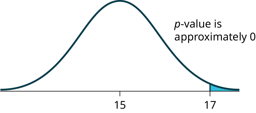
Suppose the null hypothesis is true (the mean height of the loaves is no more than 15 cm). Then is the mean height (17 cm) calculated from the sample unexpectedly large? The hypothesis test works by asking the question how unlikely the sample mean would be if the null hypothesis were true. The graph shows how far out the sample mean is on the normal curve. The p-value is the probability that, if we were to take other samples, any other sample mean would fall at least as far out as 17 cm.
The p-value, then, is the probability that a sample mean is the same or greater than 17 cm. when the population mean is, in fact, 15 cm. We can calculate this probability using the normal distribution for means.
Figure 9.2 — 9.4 Rare Events, the Sample, Decision and Conclusion
A p-value of approximately zero tells us that it is highly unlikely that a loaf of bread rises no more than 15 cm, on average. That is, almost 0% of all loaves of bread would be at least as high as 17 cm. purely by CHANCE had the population mean height really been 15 cm. Because the outcome of 17 cm. is so unlikely (meaning it is happening NOT by chance alone), we conclude that the evidence is strongly against the null hypothesis (the mean height is at most 15 cm.). There is sufficient evidence that the true mean height for the population of the baker's loaves of bread is greater than 15 cm.
Try It
9.9
A normal distribution has a standard deviation of 1. We want to verify a claim that the mean is greater than 12. A sample of 36 is taken with a sample mean of 12.5.
H0: μ ≤ 12
Ha: μ > 12
The p-value is 0.0013
Draw a graph that shows the p-value.
Decision and Conclusion
A systematic way to make a decision of whether to reject or not reject the null hypothesis
is to compare the p-value and a preset or preconceived α (also called a "significance level"). A preset α is the probability of a Type I error (rejecting the null hypothesis when the null hypothesis is true). It may or may not be given to you at the beginning of the problem.
When you make a decision to reject or not reject H0, do as follows:
If α > p-value, reject H0. The results of the sample data are significant. There is sufficient evidence to conclude that H0 is an incorrect belief and that the alternative hypothesis, Ha, may be correct.
If α ≤ p-value, do not reject H0. The results of the sample data are not significant.There is not sufficient evidence to conclude that the alternative hypothesis,Ha, may be correct.
When you "do not reject H0", it does not mean that you should believe that H0 is true. It simply means that the sample data have failed to provide sufficient evidence to cast serious doubt about the truthfulness of Ho.
Conclusion: After you make your decision, write a thoughtful conclusion about the hypotheses in terms of the given problem.
Example
9.10
When using the p-value to evaluate a hypothesis test, it is sometimes useful to use the following memory device
If the p-value is low, the null must go.
If the p-value is high, the null must fly.
This memory aid relates a p-value less than the established alpha (the p is low) as rejecting the null hypothesis and, likewise, relates a p-value higher than the established alpha (the p is high) as not rejecting the null hypothesis.
Problem
Fill in the blanks.
Reject the null hypothesis when ______________________________________.
The results of the sample data _____________________________________.
Do not reject the null when hypothesis when __________________________________________.
The results of the sample data ____________________________________________.
Reject the null hypothesis when the p-value is less than the established alpha value. The results of the sample data support the alternative hypothesis.
Do not reject the null hypothesis when the p-value is greater than the established alpha value. The results of the sample data do not support the alternative hypothesis.
Try It
9.10
It’s a Boy Genetics Labs claim their procedures improve the chances of a boy being born. The results for a test of a single population proportion are as follows:
H0: p = 0.50, Ha: p > 0.50
α = 0.01
p-value = 0.025
Interpret the results and state a conclusion in simple, non-technical terms.
2.5 Measures of the Center of the Data
OpenStax · 2.5 Measures of the Center of the Data ↗ Instructional page including learning objectives, examples, figures, source tables and questions. Site navigation and embedded media players are omitted; source media links remain available.
The "center" of a data set is also a way of describing location.
The two most widely used measures of the "center" of the data are the mean (average) and the median. To calculate the mean weight of 50 people, add the 50 weights together and divide by 50. To find the median weight of the 50 people, order the data and find the number that splits the data into two equal parts. The median is generally a better measure of the center when there are extreme values or outliers because it is not affected by the precise numerical values of the outliers. The mean is the most common measure of the center.
NOTE
The words “mean” and “average” are often used interchangeably. The substitution of one word for the other is common practice. The technical term is “arithmetic mean” and “average” is technically a center location. However, in practice among non-statisticians, “average" is commonly accepted for “arithmetic mean.”
When each value in the data set is not unique, the mean can be calculated by multiplying each distinct value by its frequency and then dividing the sum by the total number of data values. The letter used to represent the sample mean is an x with a bar over it (pronounced “x bar”): .
The Greek letter μ (pronounced "mew") represents the population mean. One of the requirements for the sample mean to be a good estimate of the population mean is for the sample taken to be truly random.
To see that both ways of calculating the mean are the same, consider the sample:
1; 1; 1; 2; 2; 3; 4; 4; 4; 4; 4
In the second calculation, the frequencies are 3, 2, 1, and 5.
You can quickly find the location of the median by using the expression .
The letter n is the total number of data values in the sample. If n is an odd number, the median is the middle value of the ordered data (ordered smallest to largest). If n is an even number, the median is equal to the two middle values added together and divided by two after the data has been ordered. For example, if the total number of data values is 97, then =
= 49. The median is the 49th value in the ordered data. If the total number of data values is 100, then =
= 50.5. The median occurs midway between the 50th and 51st values. The location of the median and the value of the median are not the same. The upper case letter M is often used to represent the median. The next example illustrates the location of the median and the value of the median.
Example
2.26
Problem
A hospital administrator keeps track of the ages (in years) of patients visiting the emergency room over a one-week period (data are sorted from smallest to largest): 3; 4; 8; 8; 10; 11; 12; 13; 14; 15; 15; 16; 16; 17; 17; 18; 21; 22; 22; 24; 24; 25; 26; 26; 27; 27; 29; 29; 31; 32; 33; 33; 34; 34; 35; 37; 40; 44; 44; 47;
Calculate the mean and the median.
To find the median, M, first use the formula for the location. The location is:
Starting at the smallest value, the median is located between the 20th and 21st values (the two 24s):
3; 4; 8; 8; 10; 11; 12; 13; 14; 15; 15; 16; 16; 17; 17; 18; 21; 22; 22; 24; 24; 25; 26; 26; 27; 27; 29; 29; 31; 32; 33; 33; 34; 34; 35; 37; 40; 44; 44; 47;
Using the TI-83, 83+, 84, 84+ Calculator
To find the mean and the median:
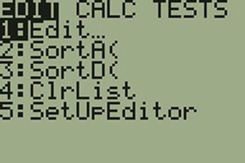
Clear list L1. Pres STAT 4:ClrList. Enter 2nd 1 for list L1. Press ENTER.
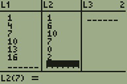
Enter data into the list editor. Press STAT 1:EDIT.
Put the data values into list L1.
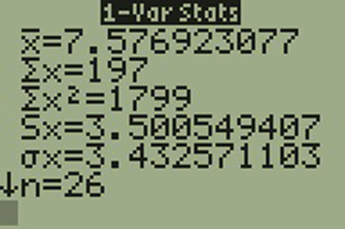
Press STAT and arrow to CALC. Press 1:1-VarStats. Press 2nd 1 for L1 and then ENTER.
Press the down and up arrow keys to scroll.
= 23.6, M = 24
Try It
2.26
The following data show the number of months patients typically wait on a transplant list before getting surgery. The data are ordered from smallest to largest. Calculate the mean and median.
Suppose that in a small town of 50 people, one person earns $5,000,000 per year and the other 49 each earn $30,000. Which is the better measure of the "center": the mean or the median?
(There are 49 people who earn $30,000 and one person who earns $5,000,000.)
The median is a better measure of the "center" than the mean because 49 of the values are 30,000 and one is 5,000,000. The 5,000,000 is an outlier. The 30,000 gives us a better sense of the middle of the data.
Try It
2.27
In a sample of 60 households, one house is worth $2,500,000. Twenty-nine houses are worth $280,000, and all the others are worth $315,000. Which is the better measure of the “center”: the mean or the median?
Another measure of the center is the mode. The mode is the most frequent value. There can be more than one mode in a data set as long as those values have the same frequency and that frequency is the highest. A data set with two modes is called bimodal.
Example
2.28
Statistics exam scores for 20 students are as follows:
Five real estate exam scores are 430, 430, 480, 480, 495. The data set is bimodal because the scores 430 and 480 each occur twice.
When is the mode the best measure of the "center"? Consider a weight loss program that advertises a mean weight loss of six pounds the first week of the program. The mode might indicate that most people lose two pounds the first week, making the program less appealing.
NOTE
The mode can be calculated for qualitative data as well as for quantitative data. For example, if the data set is: red, red, red, green, green, yellow, purple, black, blue, the mode is red.
Statistical software will easily calculate the mean, the median, and the mode. Some graphing calculators can also make these calculations. In the real world, people make these calculations using software.
Try It
2.29
Five credit scores are 680, 680, 700, 720, 720. The data set is bimodal because the scores 680 and 720 each occur twice. Consider the annual earnings of workers at a factory. The mode is $25,000 and occurs 150 times out of 301. The median is $50,000 and the mean is $47,500. What would be the best measure of the “center”?
The Law of Large Numbers and the Mean
The Law of Large Numbers says that if you take samples of larger and larger size from any population, then the mean of the sample is very likely to get closer and closer to µ. This is discussed in more detail later in the text.
Sampling Distributions and Statistic of a Sampling Distribution
You can think of a sampling distribution as a relative frequency distribution with a great many samples. (See Sampling and Data for a review of relative frequency). Suppose thirty randomly selected students were asked the number of movies they watched the previous week. The results are in the relative frequency table shown below.
# of movies
Relative Frequency
0
1
2
3
4
Table
2.25
If you let the number of samples get very large (say, 300 million or more), the relative frequency table becomes a relative frequency distribution.
A statistic is a number calculated from a sample. Statistic examples include the mean, the median and the mode as well as others. The sample mean is an example of a statistic which estimates the population mean μ.
Calculating the Mean of Grouped Frequency Tables
When only grouped data is available, you do not know the individual data values (we only know intervals and interval frequencies); therefore, you cannot compute an exact mean for the data set. What we must do is estimate the actual mean by calculating the mean of a frequency table. A frequency table is a data representation in which grouped data is displayed along with the corresponding frequencies. To calculate the mean from a grouped frequency table we can apply the basic definition of mean: mean = We simply need to modify the definition to fit within the restrictions of a frequency table.
Since we do not know the individual data values we can instead find the midpoint of each interval. The midpoint is . We can now modify the mean definition to be where f = the frequency of the interval and m = the midpoint of the interval.
Example
2.30
Problem
A frequency table displaying professor Blount’s last statistic test is shown. Find the best estimate of the class mean.
Calculate the sum of the product of each interval frequency and midpoint.
Try It
2.30
A researcher conducted a study on the effect that playing video games has on memory recall. As part of the study, they compiled the following data:
Hours Teenagers Spend on Video Games
Number of Teenagers
0–3.5
3
3.5–7.5
7
7.5–11.5
12
11.5–15.5
7
15.5–19.5
9
Table
2.28
What is the best estimate for the mean number of hours spent playing video games?
2.7 Measures of the Spread of the Data
OpenStax · 2.7 Measures of the Spread of the Data ↗ Instructional page including learning objectives, examples, figures, source tables and questions. Site navigation and embedded media players are omitted; source media links remain available.
An important characteristic of any set of data is the variation in the data. In some data sets, the data values are concentrated closely near the mean; in other data sets, the data values are more widely spread out from the mean. The most common measure of variation, or spread, is the standard deviation. The standard deviation is a number that measures how far data values are from their mean.
provides a numerical measure of the overall amount of variation in a data set, and
can be used to determine whether a particular data value is close to or far from the mean.
The standard deviation provides a measure of the overall variation in a data set
The standard deviation is always positive or zero. The standard deviation is small when the data are all concentrated close to the mean, exhibiting little variation or spread. The standard deviation is larger when the data values are more spread out from the mean, exhibiting more variation.
Suppose that we are studying the amount of time customers wait in line at the checkout at supermarket A and supermarket B. The average wait time at both supermarkets is five minutes. At supermarket A, the standard deviation for the wait time is two minutes; at supermarket B the standard deviation for the wait time is four minutes.
Because supermarket B has a higher standard deviation, we know that there is more variation in the wait times at supermarket B. Overall, wait times at supermarket B are more spread out from the average; wait times at supermarket A are more concentrated near the average.
The standard deviation can be used to determine whether a data value is close to or far from the mean.
Suppose that Rosa and Binh both shop at supermarket A. Rosa waits at the checkout counter for seven minutes and Binh waits for one minute. At supermarket A, the mean waiting time is five minutes and the standard deviation is two minutes. The standard deviation can be used to determine whether a data value is close to or far from the mean.
Rosa waits for seven minutes:
Seven is two minutes longer than the average of five; two minutes is equal to one standard deviation.
Rosa's wait time of seven minutes is two minutes longer than the average of five minutes.
Rosa's wait time of seven minutes is one standard deviation above the average of five minutes.
Binh waits for one minute.
One is four minutes less than the average of five; four minutes is equal to two standard deviations.
Binh's wait time of one minute is four minutes less than the average of five minutes.
Binh's wait time of one minute is two standard deviations below the average of five minutes.
A data value that is two standard deviations from the average is just on the borderline for what many statisticians would consider to be far from the average. Considering data to be far from the mean if it is more than two standard deviations away is more of an approximate "rule of thumb" than a rigid rule. In general, the shape of the distribution of the data affects how much of the data is further away than two standard deviations. (You will learn more about this in later chapters.)
The number line may help you understand standard deviation. If we were to put five and seven on a number line, seven is to the right of five. We say, then, that seven is onestandard deviation to the right of five because 5 + (1)(2) = 7.
If one were also part of the data set, then one is two standard deviations to the left of five because 5 + (–2)(2) = 1.
Figure 2.24 — 2.7 Measures of the Spread of the Data
If x is a number, then the difference "x – mean" is called its deviation. In a data set, there are as many deviations as there are items in the data set. The deviations are used to calculate the standard deviation. If the numbers belong to a population, in symbols a deviation is x – μ. For sample data, in symbols a deviation is x – .
The procedure to calculate the standard deviation depends on whether the numbers are the entire population or are data from a sample. The calculations are similar, but not identical. Therefore the symbol used to represent the standard deviation depends on whether it is calculated from a population or a sample. The lower case letter s represents the sample standard deviation and the Greek letter σ (sigma, lower case) represents the population standard deviation. If the sample has the same characteristics as the population, then s should be a good estimate of σ.
To calculate the standard deviation, we need to calculate the variance first. The variance is the average of the squares of the deviations (the x – values for a sample, or the x – μ values for a population). The symbol σ2 represents the population variance; the population standard deviationσ is the square root of the population variance. The symbol s2 represents the sample variance; the sample standard deviations is the square root of the sample variance. You can think of the standard deviation as a special average of the deviations.
If the numbers come from a census of the entire population and not a sample, when we calculate the average of the squared deviations to find the variance, we divide by N, the number of items in the population. If the data are from a sample rather than a population, when we calculate the average of the squared deviations, we divide by n – 1, one less than the number of items in the sample.
For the population standard deviation, the denominator is N, the number of items in the population.
In these formulas, f represents the frequency with which a value appears. For example, if a value appears once, f is one. If a value appears three times in the data set or population, f is three.
In practice, USE A CALCULATOR OR COMPUTER SOFTWARE TO CALCULATE THE STANDARD DEVIATION. If you are using a TI-83, 83+, 84+ calculator, you need to select the appropriate standard deviationσx or sx from the summary statistics. We will concentrate on using and interpreting the information that the standard deviation gives us. However you should study the following step-by-step example to help you understand how the standard deviation measures variation from the mean. (The calculator instructions appear at the end of this example.)
Example
2.32
In a fifth grade class, the teacher was interested in the average age and the sample standard deviation of the ages of the students. The following data are the ages for a SAMPLE of n = 20 fifth grade students. The ages are rounded to the nearest half year:
The average age is 10.53 years, rounded to two places.
The variance may be calculated by using a table. Then the standard deviation is calculated by taking the square root of the variance. We will explain the parts of the table after calculating s.
Data
Freq.
Deviations
Deviations2
(Freq.)(Deviations2)
x
f
(x – )
(x – )2
(f)(x – )2
9
1
9 – 10.525 = –1.525
(–1.525)2 = 2.325625
1 × 2.325625 = 2.325625
9.5
2
9.5 – 10.525 = –1.025
(–1.025)2 = 1.050625
2 × 1.050625 = 2.101250
10
4
10 – 10.525 = –0.525
(–0.525)2 = 0.275625
4 × 0.275625 = 1.1025
10.5
4
10.5 – 10.525 = –0.025
(–0.025)2 = 0.000625
4 × 0.000625 = 0.0025
11
6
11 – 10.525 = 0.475
(0.475)2 = 0.225625
6 × 0.225625 = 1.35375
11.5
3
11.5 – 10.525 = 0.975
(0.975)2 = 0.950625
3 × 0.950625 = 2.851875
The total is 9.7375
Table
2.30
The sample variance, s2, is equal to the sum of the last column (9.7375) divided by the total number of data values minus one (20 – 1):
The sample standard deviations is equal to the square root of the sample variance:
which is rounded to two decimal places, s = 0.72.
Typically, you do the calculation for the standard deviation on your calculator or computer. The intermediate results are not rounded. This is done for accuracy.
Problem
For the following problems, recall that value = mean + (#ofSTDEVs)(standard deviation). Verify the mean and standard deviation or a calculator or computer.
The deviations show how spread out the data are about the mean. The data value 11.5 is farther from the mean than is the data value 11 which is indicated by the deviations 0.97 and 0.47. A positive deviation occurs when the data value is greater than the mean, whereas a negative deviation occurs when the data value is less than the mean. The deviation is –1.525 for the data value nine. If you add the deviations, the sum is always zero. (For Example 2.32, there are n = 20 deviations.) So you cannot simply add the deviations to get the spread of the data. By squaring the deviations, you make them positive numbers, and the sum will also be positive. The variance, then, is the average squared deviation.
The variance is a squared measure and does not have the same units as the data. Taking the square root solves the problem. The standard deviation measures the spread in the same units as the data.
Notice that instead of dividing by n = 20, the calculation divided by n – 1 = 20 – 1 = 19 because the data is a sample. For the sample variance, we divide by the sample size minus one (n – 1). Why not divide by n? The answer has to do with the population variance. The sample variance is an estimate of the population variance. Based on the theoretical mathematics that lies behind these calculations, dividing by (n – 1) gives a better estimate of the population variance.
NOTE
Your concentration should be on what the standard deviation tells us about the data. The standard deviation is a number which measures how far the data are spread from the mean. Let a calculator or computer do the arithmetic.
The standard deviation, s or σ, is either zero or larger than zero. Describing the data with reference to the spread is called "variability". The variability in data depends upon the method by which the outcomes are obtained; for example, by measuring or by random sampling. When the standard deviation is zero, there is no spread; that is, the all the data values are equal to each other. The standard deviation is small when the data are all concentrated close to the mean, and is larger when the data values show more variation from the mean. When the standard deviation is a lot larger than zero, the data values are very spread out about the mean; outliers can make s or σ very large.
The standard deviation, when first presented, can seem unclear. By graphing your data, you can get a better "feel" for the deviations and the standard deviation. You will find that in symmetrical distributions, the standard deviation can be very helpful but in skewed distributions, the standard deviation may not be much help. The reason is that the two sides of a skewed distribution have different spreads. In a skewed distribution, it is better to look at the first quartile, the median, the third quartile, the smallest value, and the largest value. Because numbers can be confusing, always graph your data. Display your data in a histogram or a box plot.
Example
2.33
Problem
Use the following data (first exam scores) from Professor Dean's spring pre-calculus class:
The x-axis goes from 32.5 to 100.5; y-axis goes from –2.4 to 15 for the histogram. The number of intervals is five, so the width of an interval is (100.5 – 32.5) divided by five, is equal to 13.6. Endpoints of the intervals are as follows: the starting point is 32.5, 32.5 + 13.6 = 46.1, 46.1 + 13.6 = 59.7, 59.7 + 13.6 = 73.3, 73.3 + 13.6 = 86.9, 86.9 + 13.6 = 100.5 = the ending value; No data values fall on an interval boundary.
Figure 2.25 — 2.7 Measures of the Spread of the Data
The long left whisker in the box plot is reflected in the left side of the histogram. The spread of the exam scores in the lower 50% is greater (73 – 33 = 40) than the spread in the upper 50% (100 – 73 = 27). The histogram, box plot, and chart all reflect this. There are a substantial number of A and B grades (80s, 90s, and 100). The histogram clearly shows this. The box plot shows us that the middle 50% of the exam scores (IQR = 29) are Ds, Cs, and Bs. The box plot also shows us that the lower 25% of the exam scores are Ds and Fs.
Try It
2.33
The following data show the different types of pet food stores in the area carry.
6; 6; 6; 6; 7; 7; 7; 7; 7; 8; 9; 9; 9; 9; 10; 10; 10; 10; 10; 11; 11; 11; 11; 12; 12; 12; 12; 12; 12;
Calculate the sample mean and the sample standard deviation to one decimal place using a TI-83+ or TI-84 calculator.
Recall that for grouped data we do not know individual data values, so we cannot describe the typical value of the data with precision. In other words, we cannot find the exact mean, median, or mode. We can, however, determine the best estimate of the measures of center by finding the mean of the grouped data with the formula:
where interval frequencies and m = interval midpoints.
Just as we could not find the exact mean, neither can we find the exact standard deviation. Remember that standard deviation describes numerically the expected deviation a data value has from the mean. In simple English, the standard deviation allows us to compare how “unusual” individual data is compared to the mean.
The values in the second, third, and fourth columns of Table 2.32 are used to calculate the mean of the grouped frequency table, the value in the fifth column.
After calculating , find the difference, , for each midpoint, . Next, square each difference. In the final column, calculate the product of the frequency and the squared difference for each class.
The table makes it easy to use the formula for calculating the standard deviation of a grouped frequency table:
Although the formula is not complicated, these calculations are typically performed using technology.
The standard deviation is useful when comparing data values that come from different data sets. If the data sets have different means and standard deviations, then comparing the data values directly can be misleading.
For each data value, calculate how many standard deviations away from its mean the value is.
Use the formula: value = mean + (#ofSTDEVs)(standard deviation); solve for #ofSTDEVs.
Compare the results of this calculation.
#ofSTDEVs is often called a "z-score"; we can use the symbol z. In symbols, the formulas become:
Sample
= + zs
Population
= + zσ
Table
2.34
Example
2.35
Problem
Two students, John and Ali, from different high schools, wanted to find out who had the highest GPA when compared to his school. Which student had the highest GPA when compared to his school?
For each student, determine how many standard deviations (#ofSTDEVs) his GPA is away from the average, for his school. Pay careful attention to signs when comparing and interpreting the answer.
For John,
For Ali,
John has the better GPA when compared to his school because his GPA is 0.21 standard deviations belowhis school's mean while Ali's GPA is 0.3 standard deviations belowhis school's mean.
John's z-score of –0.21 is higher than Ali's z-score of –0.3. For GPA, higher values are better, so we conclude that John has the better GPA when compared to his school.
Try It
2.35
Two swimmers, Angie and Beth, from different teams, wanted to find out who had the fastest time for the 50 meter freestyle when compared to her team. Which swimmer had the fastest time when compared to her team?
The following lists give a few facts that provide a little more insight into what the standard deviation tells us about the distribution of the data.
For ANY data set, no matter what the distribution of the data is:
At least 75% of the data is within two standard deviations of the mean.
At least 89% of the data is within three standard deviations of the mean.
At least 95% of the data is within 4.5 standard deviations of the mean.
This is known as Chebyshev's Rule.
For data having a distribution that is BELL-SHAPED and SYMMETRIC:
Approximately 68% of the data is within one standard deviation of the mean.
Approximately 95% of the data is within two standard deviations of the mean.
More than 99% of the data is within three standard deviations of the mean.
This is known as the Empirical Rule.
It is important to note that this rule only applies when the shape of the distribution of the data is bell-shaped and symmetric. We will learn more about this when studying the "Normal" or "Gaussian" probability distribution in later chapters.
8.1 A Single Population Mean using the Normal Distribution
A confidence interval for a population mean, when the population standard deviation is known, is based on the conclusion of the Central Limit Theorem that the sampling distribution of the sample means follow an approximately normal distribution. Suppose that our sample has a mean of and we have constructed the 90% confidence interval (5, 15) where EBM = 5.
To construct a confidence interval for a single unknown population mean μ, where the population standard deviation is known, we need as an estimate for μ and we need the margin of error. Here, the margin of error (EBM) is called the error bound for a population mean (abbreviated EBM). The sample mean is the point estimate of the unknown population mean μ.
(point estimate - error bound, point estimate + error bound) or, in symbols,()
The margin of error (EBM) depends on the confidence level (abbreviated CL). The confidence level is often considered the probability that the calculated confidence interval estimate will contain the true population parameter. However, it is more accurate to state that the confidence level is the percent of confidence intervals that contain the true population parameter when repeated samples are taken. Most often, it is the choice of the person constructing the confidence interval to choose a confidence level of 90% or higher because that person wants to be reasonably certain of their conclusions.
There is another probability called alpha (α). α is related to the confidence level, CL. α is the probability that the interval does not contain the unknown population parameter.
Mathematically, α + CL = 1.
Example
8.1
Suppose we have collected data from a sample. We know the sample mean but we do not know the mean for the entire population.
The sample mean is seven, and the error bound for the mean is 2.5.
= 7 and EBM = 2.5
The confidence interval is (7 – 2.5, 7 + 2.5), and calculating the values gives (4.5, 9.5).
If the confidence level (CL) is 95%, then we say that, "We estimate with 95% confidence that the true value of the population mean is between 4.5 and 9.5."
Try It
8.1
Suppose we have data from a sample. The sample mean is 15, and the error bound for the mean is 3.2.
A confidence interval for a population mean with a known standard deviation is based on the fact that the sample means follow an approximately normal distribution. Suppose that our sample has a mean of , and we have constructed the 90% confidence interval (1.8, 2.2) where EBM = 0.1.
To get a 90% confidence interval, we must include the central 90% of the probability of the normal distribution. If we include the central 90%, we leave out a total of α = 10% in both tails, or 5% in each tail, of the normal distribution.
Figure 8.2 — 8.1 A Single Population Mean using the Normal Distribution
To capture the central 90%, we must go out 1.645 "standard deviations" on either side of the calculated sample mean. The value 1.645 is the z-score from a standard normal probability distribution that puts an area of 0.90 in the center, an area of 0.05 in the far left tail, and an area of 0.05 in the far right tail.
To construct a confidence interval estimate for an unknown population mean, we need data from a random sample. The steps to construct and interpret the confidence interval are:
Calculate the sample mean from the sample data. Remember, in this section we already know the population standard deviationσ.
Find the z-score that corresponds to the confidence level.
Write a sentence that interprets the estimate in the context of the situation in the problem. (Explain what the confidence interval means, in the words of the problem.)
We will first examine each step in more detail, and then illustrate the process with some examples.
Finding the z-score for the Stated Confidence Level
When we know the population standard deviationσ, we use a standard normal distribution to calculate the error bound EBM and construct the confidence interval. We need to find the value of z that puts an area equal to the confidence level (in decimal form) in the middle of the standard normal distribution Z ~ N(0, 1).
The confidence level, CL, is the area in the middle of the standard normal distribution. CL = 1 – α, so α is the area that is split equally between the two tails. Each of the tails contains an area equal to .
The z-score that has an area to the right of is denoted by .
For example, when CL = 0.95, α = 0.05 and = 0.025; we write = z0.025.
The area to the right of z0.025 is 0.025 and the area to the left of z0.025 is 1 – 0.025 = 0.975.
, using a calculator, computer or a standard normal probability table.
Using the TI-83, 83+, 84, 84+ Calculator
invNorm(0.975, 0, 1) = 1.96
NOTE
Remember to use the area to the LEFT of ; in this chapter the last two inputs in the invNorm command are 0, 1, because you are using a standard normal distribution Z ~ N(0, 1).
Writing the Interpretation
The interpretation should clearly state the confidence level (CL), explain what population parameter is being estimated (here, a population mean), and state the confidence interval (both endpoints). "We estimate with ___% confidence that the true population mean (include the context of the problem) is between ___ and ___ (include appropriate units)."
Example
8.2
Suppose scores on exams in statistics are normally distributed with an unknown population mean and a population standard deviation of three points. A random sample of 36 scores is taken and gives a sample mean (sample mean score) of 68. Find a confidence interval estimate for the population mean exam score (the mean score on all exams).
Problem
Find a 90% confidence interval for the true (population) mean of statistics exam scores.
For a 90% confidence interval, visualize an area of 0.90 centered under the normal curve (See Figure 8.3). The remaining area for the two tails of the normal distribution is then 0.10, which indicates that the area in the left tail is one-half of 0.10, which is 0.05. The corresponding z-score that cuts off an area of 0.05 in the left tail is 1.645.
Press STAT and arrow over to TESTS.
Arrow down to 7:ZInterval.
Press ENTER.
Arrow to Stats and press ENTER.
Arrow down and enter three for σ, 68 for , 36 for n, and .90 for C-level.
Arrow down to Calculate and press ENTER.
The confidence interval is (to three decimal places)(67.178, 68.822).
Explanation of 90% Confidence Level:
Ninety percent of all confidence intervals constructed in this way contain the true mean statistics exam score. For example, if we constructed 100 of these confidence intervals, we would expect 90 of them to contain the true population mean exam score.
Try It
8.2
Suppose average pizza delivery times are normally distributed with an unknown population mean and a population standard deviation of six minutes. A random sample of 28 pizza delivery restaurants is taken and has a sample mean delivery time of 36 minutes.
Find a 90% confidence interval estimate for the population mean delivery time.
Example
8.3
The Specific Absorption Rate (SAR) for a cell phone measures the amount of radio frequency (Rf) energy absorbed by the user’s body when using the handset. Every cell phone emits Rf energy. Different phone models have different SAR measures. To receive certification from the Federal Communications Commission (FCC) for sale in the United States, the SAR level for a cell phone must be no more than 1.6 watts per kilogram. Table 8.1 shows the highest SAR level for a random selection of cell phone models as measured by the FCC.
SAR Data for a sample of 30 cell phones
1.11
1.36
0.74
1.48
1.34
0.5
1.43
1.18
0.4
1.3
1.3
0.867
1.09
1.26
0.68
0.455
1.29
0.51
1.41
0.36
1.13
0.82
0.52
0.3
0.78
1.6
1.48
1.25
1.39
1.38
Table
8.1
Problem
Find a 98% confidence interval for the true (population) mean of the Specific Absorption Rates (SARs) for cell phones. Assume that the population standard deviation is σ = 0.337.
You need to find z0.01 having the property that the area under the normal density curve to the right of z0.01 is 0.01 and the area to the left is 0.99. Use your calculator, a computer, or a probability table for the standard normal distribution to find z0.01 = 2.326.
We estimate with 98% confidence that the true SAR mean for the population of cell phones in the United States is between 0.8809 and 1.1671 watts per kilogram.
Table 8.2 shows a different random sampling of 20 cell phone models. Use this data to calculate a 93% confidence interval for the true mean SAR for cell phones certified for use in the United States. As previously, assume that the population standard deviation is σ = 0.337.
SAR Data for a sample of 20 cell phones
1.48
1.53
0.8
0.68
1.15
1.4
1.36
1.24
0.77
0.57
0.462
0.2
1.36
0.51
1.39
0.3
1.3
0.73
0.7
0.869
Table
8.2
Notice the difference in the confidence intervals calculated in Example 8.3 and the following Try It exercise. These intervals are different for several reasons: they were calculated from different samples, the samples were different sizes, and the intervals were calculated for different levels of confidence. Even though the intervals are different, they do not yield conflicting information. The effects of these kinds of changes are the subject of the next section in this chapter.
Changing the Confidence Level or Sample Size
Example
8.4
Problem
Suppose we change the original problem in Example 8.2 by using a 95% confidence level. Find a 95% confidence interval for the true (population) mean statistics exam score.
σ = 3; n = 36; The confidence level is 95% (CL = 0.95).
CL = 0.95 so α = 1 – CL = 1 – 0.95 = 0.05
The area to the right of z0.025 is 0.025 and the area to the left of z0.025 is 1 – 0.025 = 0.975.
when using invnorm(0.975,0,1) on the TI-83, 83+, or 84+ calculators. (This can also be found using appropriate commands on other calculators, using a computer, or using a probability table for the standard normal distribution.)
EBM = (1.96) = 0.98
– EBM = 68 – 0.98 = 67.02
+ EBM = 68 + 0.98 = 68.98
Notice that the EBM is larger for a 95% confidence level in the original problem.
We estimate with 95% confidence that the true population mean for all statistics exam scores is between 67.02 and 68.98.
Explanation of 95% Confidence Level:
Ninety-five percent of all confidence intervals constructed in this way contain the true value of the population mean statistics exam score.
Comparing the results:
The 90% confidence interval is (67.18, 68.82). The 95% confidence interval is (67.02, 68.98). The 95% confidence interval is wider. If you look at the graphs, because the area 0.95 is larger than the area 0.90, it makes sense that the 95% confidence interval is wider. To be more confident that the confidence interval actually does contain the true value of the population mean for all statistics exam scores, the confidence interval necessarily needs to be wider.
Figure 8.5 — 8.1 A Single Population Mean using the Normal Distribution
Increasing the confidence level increases the error bound, making the confidence interval wider.
Decreasing the confidence level decreases the error bound, making the confidence interval narrower.
Try It
8.4
Refer back to the pizza-delivery Try It exercise. The population standard deviation is six minutes and the sample mean deliver time is 36 minutes. Use a sample size of 20. Find a 95% confidence interval estimate for the true mean pizza delivery time.
Example
8.5
Suppose we change the original problem in Example 8.2 to see what happens to the error bound if the sample size is changed.
Problem
Leave everything the same except the sample size. Use the original 90% confidence level. What happens to the error bound and the confidence interval if we increase the sample size and use n = 100 instead of n = 36? What happens if we decrease the sample size to n = 25 instead of n = 36?
= 68
EBM =
σ = 3; The confidence level is 90% (CL=0.90); = z0.05 = 1.645.
If we decrease the sample size n to 25, we increase the error bound.
When n = 25: EBM = = (1.645) = 0.987.
Summary: Effect of Changing the Sample Size
Increasing the sample size causes the error bound to decrease, making the confidence interval narrower.
Decreasing the sample size causes the error bound to increase, making the confidence interval wider.
Try It
8.5
Refer back to the pizza-delivery Try It exercise. The mean delivery time is 36 minutes and the population standard deviation is six minutes. Assume the sample size is changed to 50 restaurants with the same sample mean. Find a 90% confidence interval estimate for the population mean delivery time.
Working Backwards to Find the Error Bound or Sample Mean
When we calculate a confidence interval, we find the sample mean, calculate the error bound, and use them to calculate the confidence interval. However, sometimes when we read statistical studies, the study may state the confidence interval only. If we know the confidence interval, we can work backwards to find both the error bound and the sample mean.
Finding the Error Bound
From the upper value for the interval, subtract the sample mean,
OR, from the upper value for the interval, subtract the lower value. Then divide the difference by two.
Notice that there are two methods to perform each calculation. You can choose the method that is easier to use with the information you know.
Example
8.6
Suppose we know that a confidence interval is (67.18, 68.82) and we want to find the error bound. We may know that the sample mean is 68, or perhaps our source only gave the confidence interval and did not tell us the value of the sample mean.
Calculate the Error Bound:
If we know that the sample mean is 68: EBM = 68.82 – 68 = 0.82.
If we don't know the sample mean: EBM = = 0.82.
Calculate the Sample Mean:
If we know the error bound:
= 68.82 – 0.82 = 68
If we don't know the error bound: = = 68.
Try It
8.6
Suppose we know that a confidence interval is (42.12, 47.88). Find the error bound and the sample mean.
Calculating the Sample Size n
If researchers desire a specific margin of error, then they can use the error bound formula to calculate the required sample size.
The error bound formula for a population mean when the population standard deviation is known is EBM = .
The formula for sample size is n = , found by solving the error bound formula for n.
In this formula, z is , corresponding to the desired confidence level. A researcher planning a study who wants a specified confidence level and error bound can use this formula to calculate the size of the sample needed for the study.
Example
8.7
The population standard deviation for the age of Foothill College students is 15 years. If we want to be 95% confident that the sample mean age is within two years of the true population mean age of Foothill College students, how many randomly selected Foothill College students must be surveyed?
From the problem, we know that σ = 15 and EBM = 2.
z = z0.025 = 1.96, because the confidence level is 95%.
n = = = 216.09 using the sample size equation.
Use n = 217: Always round the answer UP to the next higher integer to ensure that the sample size is large enough.
Therefore, 217 Foothill College students should be surveyed in order to be 95% confident that we are within two years of the true population mean age of Foothill College students.
Try It
8.7
The population standard deviation for the height of high school basketball players is three inches. If we want to be 95% confident that the sample mean height is within one inch of the true population mean height, how many randomly selected students must be surveyed?
2.3 Analyzing Findings
OpenStax · 2.3 Analyzing Findings ↗ Instructional page including learning objectives, examples, figures, source tables and questions. Site navigation and embedded media players are omitted; source media links remain available.
Learning Objectives
By the end of this section, you will be able to:
Explain what a correlation coefficient tells us about the relationship between variables
Recognize that correlation does not indicate a cause-and-effect relationship between variables
Discuss our tendency to look for relationships between variables that do not really exist
Explain random sampling and assignment of participants into experimental and control groups
Discuss how experimenter or participant bias could affect the results of an experiment
Identify independent and dependent variables
Did you know that as sales in ice cream increase, so does the overall rate of crime? Is it possible that indulging in your favorite flavor of ice cream could send you on a crime spree? Or, after committing crime do you think you might decide to treat yourself to a cone? There is no question that a relationship exists between ice cream and crime (e.g., Harper, 2013), but it would be pretty foolish to decide that one thing actually caused the other to occur.
It is much more likely that both ice cream sales and crime rates are related to the temperature outside. When the temperature is warm, there are lots of people out of their houses, interacting with each other, getting annoyed with one another, and sometimes committing crimes. Also, when it is warm outside, we are more likely to seek a cool treat like ice cream. How do we determine if there is indeed a relationship between two things? And when there is a relationship, how can we discern whether it is attributable to coincidence or causation?
Correlational Research
Correlation means that there is a relationship between two or more variables (such as ice cream consumption and crime), but this relationship does not necessarily imply cause and effect. When two variables are correlated, it simply means that as one variable changes, so does the other. We can measure correlation by calculating a statistic known as a correlation coefficient. A correlation coefficient is a number from -1 to +1 that indicates the strength and direction of the relationship between variables. The correlation coefficient is usually represented by the letter r.
The number portion of the correlation coefficient indicates the strength of the relationship. The closer the number is to 1 (be it negative or positive), the more strongly related the variables are, and the more predictable changes in one variable will be as the other variable changes. The closer the number is to zero, the weaker the relationship, and the less predictable the relationship between the variables becomes. For instance, a correlation coefficient of 0.9 indicates a far stronger relationship than a correlation coefficient of 0.3. If the variables are not related to one another at all, the correlation coefficient is 0. The example above about ice cream and crime is an example of two variables that we might expect to have no relationship to each other.
The sign—positive or negative—of the correlation coefficient indicates the direction of the relationship (Figure 2.12). A positive correlation means that the variables move in the same direction. Put another way, it means that as one variable increases so does the other, and conversely, when one variable decreases so does the other. A negative correlation means that the variables move in opposite directions. If two variables are negatively correlated, a decrease in one variable is associated with an increase in the other and vice versa.
The example of ice cream and crime rates is a positive correlation because both variables increase when temperatures are warmer. Other examples of positive correlations are the relationship between an individual’s height and weight or the relationship between a person’s age and number of wrinkles. One might expect a negative correlation to exist between someone’s tiredness during the day and the number of hours they slept the previous night: the amount of sleep decreases as the feelings of tiredness increase. In a real-world example of negative correlation, student researchers at the University of Minnesota found a weak negative correlation (r = -0.29) between the average number of days per week that students got fewer than 5 hours of sleep and their GPA (Lowry, Dean, & Manders, 2010). Keep in mind that a negative correlation is not the same as no correlation. For example, we would probably find no correlation between hours of sleep and shoe size.
As mentioned earlier, correlations have predictive value. Imagine that you are on the admissions committee of a major university. You are faced with a huge number of applications, but you are able to accommodate only a small percentage of the applicant pool. How might you decide who should be admitted? You might try to correlate your current students’ college GPA with their scores on standardized tests like the SAT or ACT. By observing which correlations were strongest for your current students, you could use this information to predict relative success of those students who have applied for admission into the university.
Figure 2.12 — 2.3 Analyzing Findings
Figure 2.12 Scatterplots are a graphical view of the strength and direction of correlations. The stronger the correlation, the closer the data points are to a straight line. In these examples, we see that there is (a) a positive correlation between weight and height, (b) a negative correlation between tiredness and hours of sleep, and (c) no correlation between shoe size and hours of sleep.
Manipulate this interactive scatterplot to practice your understanding of positive and negative correlation.
Correlation Does Not Indicate Causation
Correlational research is useful because it allows us to discover the strength and direction of relationships that exist between two variables. However, correlation is limited because establishing the existence of a relationship tells us little about cause and effect. While variables are sometimes correlated because one does cause the other, it could also be that some other factor, a confounding variable, is actually causing the systematic movement in our variables of interest. In the ice cream/crime rate example mentioned earlier, temperature is a confounding variable that could account for the relationship between the two variables.
Even when we cannot point to clear confounding variables, we should not assume that a correlation between two variables implies that one variable causes changes in another. This can be frustrating when a cause-and-effect relationship seems clear and intuitive. Think back to our discussion of the research done by the American Cancer Society and how their research projects were some of the first demonstrations of the link between smoking and cancer. It seems reasonable to assume that smoking causes cancer, but if we were limited to correlational research, we would be overstepping our bounds by making this assumption.
Unfortunately, people mistakenly make claims of causation as a function of correlations all the time. Such claims are especially common in advertisements and news stories. For example, research found that people who eat certain breakfast cereal may have a reduced risk of heart disease (Anderson, Hanna, Peng, & Kryscio, 2000). Cereal companies are likely to share this information in a way that maximizes and perhaps overstates the positive aspects of eating cereal. But does cereal really cause better health, or are there other possible explanations for the health of those who eat cereal? While correlational research is invaluable in identifying relationships among variables, a major limitation is the inability to establish causality. Psychologists want to make statements about cause and effect, but the only way to do that is to conduct an experiment to answer a research question. The next section describes how scientific experiments incorporate methods that eliminate, or control for, alternative explanations, which allow researchers to explore how changes in one variable cause changes in another variable.
Figure 2.13 — 2.3 Analyzing Findings
Figure 2.13 Does eating cereal really cause someone to be healthier? (credit: Tim Skillern)
The temptation to make erroneous cause-and-effect statements based on correlational research is not the only way we tend to misinterpret data. We also tend to make the mistake of illusory correlations, especially with unsystematic observations. Illusory correlations, or false correlations, occur when people believe that relationships exist between two things when no such relationship exists. One well-known illusory correlation is the supposed effect that the moon’s phases have on human behavior. Many people passionately assert that human behavior is affected by the phase of the moon, and specifically, that people act strangely when the moon is full (Figure 2.14).
Figure 2.14 — 2.3 Analyzing Findings
Figure 2.14 Many people believe that a full moon makes people behave oddly. (credit: Cory Zanker)
There is no denying that the moon exerts a powerful influence on our planet. The ebb and flow of the ocean’s tides are tightly tied to the gravitational forces of the moon. Many people believe, therefore, that it is logical that we are affected by the moon as well. After all, our bodies are largely made up of water. A meta-analysis of nearly 40 studies consistently demonstrated, however, that the relationship between the moon and our behavior does not exist (Rotton & Kelly, 1985). While we may pay more attention to odd behavior during the full phase of the moon, the rates of odd behavior remain constant throughout the lunar cycle.
Why are we so apt to believe in illusory correlations like this? Often we read or hear about them and simply accept the information as valid. Or, we have a hunch about how something works and then look for evidence to support that hunch, ignoring evidence that would tell us our hunch is false; this is known as confirmation bias. Other times, we find illusory correlations based on the information that comes most easily to mind, even if that information is severely limited. And while we may feel confident that we can use these relationships to better understand and predict the world around us, illusory correlations can have significant drawbacks. For example, research suggests that illusory correlations—in which certain behaviors are inaccurately attributed to certain groups—are involved in the formation of prejudicial attitudes that can ultimately lead to discriminatory behavior (Fiedler, 2004).
Causality: Conducting Experiments and Using the Data
As you’ve learned, the only way to establish that there is a cause-and-effect relationship between two variables is to conduct a scientific experiment. Experiment has a different meaning in the scientific context than in everyday life. In everyday conversation, we often use it to describe trying something for the first time, such as experimenting with a new hair style or a new food. However, in the scientific context, an experiment has precise requirements for design and implementation.
The Experimental Hypothesis
In order to conduct an experiment, a researcher must have a specific hypothesis to be tested. As you’ve learned, hypotheses can be formulated either through direct observation of the real world or after careful review of previous research. For example, if you think that the use of technology in the classroom has negative impacts on learning, then you have basically formulated a hypothesis—namely, that the use of technology in the classroom should be limited because it decreases learning. How might you have arrived at this particular hypothesis? You may have noticed that your classmates who take notes on their laptops perform at lower levels on class exams than those who take notes by hand, or those who receive a lesson via a computer program versus via an in-person teacher have different levels of performance when tested (Figure 2.15).
Figure 2.15 — 2.3 Analyzing Findings
Figure 2.15 How might the use of technology in the classroom impact learning? (credit: modification of work by Nikolay Georgiev/Pixabay)
Rose M. Spielman, William J. Jenkins, and Marilyn D. Lovett, Psychology 2E, OpenStax. (credit: modification of work by Nikolay Georgiev/Pixabay) · CC BY-NC-SA 4.0
· Original image ↗ · Access for free ↗
These sorts of personal observations are what often lead us to formulate a specific hypothesis, but we cannot use limited personal observations and anecdotal evidence to rigorously test our hypothesis. Instead, to find out if real-world data supports our hypothesis, we have to conduct an experiment.
Designing an Experiment
The most basic experimental design involves two groups: the experimental group and the control group. The two groups are designed to be the same except for one difference— experimental manipulation. The experimental group gets the experimental manipulation—that is, the treatment or variable being tested (in this case, the use of technology)—and the control group does not. Since experimental manipulation is the only difference between the experimental and control groups, we can be sure that any differences between the two are due to experimental manipulation rather than chance.
In our example of how the use of technology should be limited in the classroom, we have the experimental group learn algebra using a computer program and then test their learning. We measure the learning in our control group after they are taught algebra by a teacher in a traditional classroom. It is important for the control group to be treated similarly to the experimental group, with the exception that the control group does not receive the experimental manipulation.
We also need to precisely define, or operationalize, how we measure learning of algebra. An operational definition is a precise description of our variables, and it is important in allowing others to understand exactly how and what a researcher measures in a particular experiment. In operationalizing learning, we might choose to look at performance on a test covering the material on which the individuals were taught by the teacher or the computer program. We might also ask our participants to summarize the information that was just presented in some way. Whatever we determine, it is important that we operationalize learning in such a way that anyone who hears about our study for the first time knows exactly what we mean by learning. This aids peoples’ ability to interpret our data as well as their capacity to repeat our experiment should they choose to do so.
Once we have operationalized what is considered use of technology and what is considered learning in our experiment participants, we need to establish how we will run our experiment. In this case, we might have participants spend 45 minutes learning algebra (either through a computer program or with an in-person math teacher) and then give them a test on the material covered during the 45 minutes.
Ideally, the people who score the tests are unaware of who was assigned to the experimental or control group, in order to control for experimenter bias. Experimenter bias refers to the possibility that a researcher’s expectations might skew the results of the study. Remember, conducting an experiment requires a lot of planning, and the people involved in the research project have a vested interest in supporting their hypotheses. If the observers knew which child was in which group, it might influence how they interpret ambiguous responses, such as sloppy handwriting or minor computational mistakes. By being blind to which child is in which group, we protect against those biases. This situation is a single-blind study, meaning that one of the groups (participants) are unaware as to which group they are in (experiment or control group) while the researcher who developed the experiment knows which participants are in each group.
In a double-blind study, both the researchers and the participants are blind to group assignments. Why would a researcher want to run a study where no one knows who is in which group? Because by doing so, we can control for both experimenter and participant expectations. If you are familiar with the phrase placebo effect, you already have some idea as to why this is an important consideration. The placebo effect occurs when people's expectations or beliefs influence or determine their experience in a given situation. In other words, simply expecting something to happen can actually make it happen.
The placebo effect is commonly described in terms of testing the effectiveness of a new medication. Imagine that you work in a pharmaceutical company, and you think you have a new drug that is effective in treating depression. To demonstrate that your medication is effective, you run an experiment with two groups: The experimental group receives the medication, and the control group does not. But you don’t want participants to know whether they received the drug or not.
Why is that? Imagine that you are a participant in this study, and you have just taken a pill that you think will improve your mood. Because you expect the pill to have an effect, you might feel better simply because you took the pill and not because of any drug actually contained in the pill—this is the placebo effect.
To make sure that any effects on mood are due to the drug and not due to expectations, the control group receives a placebo (in this case a sugar pill). Now everyone gets a pill, and once again neither the researcher nor the experimental participants know who got the drug and who got the sugar pill. Any differences in mood between the experimental and control groups can now be attributed to the drug itself rather than to experimenter bias or participant expectations (Figure 2.16).
Figure 2.16 — 2.3 Analyzing Findings
Figure 2.16 Providing the control group with a placebo treatment protects against bias caused by expectancy. (credit: Elaine and Arthur Shapiro)
In a research experiment, we strive to study whether changes in one thing cause changes in another. To achieve this, we must pay attention to two important variables, or things that can be changed, in any experimental study: the independent variable and the dependent variable. An independent variable is manipulated or controlled by the experimenter. In a well-designed experimental study, the independent variable is the only important difference between the experimental and control groups. In our example of how technology use in the classroom affects learning, the independent variable is the type of learning by participants in the study (Figure 2.17). A dependent variable is what the researcher measures to see how much effect the independent variable had. In our example, the dependent variable is the learning exhibited by our participants.
Figure 2.17 — 2.3 Analyzing Findings
Figure 2.17 In an experiment, manipulations of the independent variable are expected to result in changes in the dependent variable. (credit: “classroom” modification of work by Nikolay Georgiev/Pixabay; credit “note taking”: modification of work by KF/Wikimedia)
Rose M. Spielman, William J. Jenkins, and Marilyn D. Lovett, Psychology 2E, OpenStax. (credit: “classroom” modification of work by Nikolay Georgiev/Pixabay; credit “note taking”: modification of work by KF/Wikimedia) · CC BY-NC-SA 4.0
· Original image ↗ · Access for free ↗
We expect that the dependent variable will change as a function of the independent variable. In other words, the dependent variabledepends on the independent variable. A good way to think about the relationship between the independent and dependent variables is with this question: What effect does the independent variable have on the dependent variable? Returning to our example, what is the effect of being taught a lesson through a computer program versus through an in-person instructor?
Selecting and Assigning Experimental Participants
Now that our study is designed, we need to obtain a sample of individuals to include in our experiment. Our study involves human participants so we need to determine whom to include. Participants are the subjects of psychological research, and as the name implies, individuals who are involved in psychological research actively participate in the process. Often, psychological research projects rely on college students to serve as participants. In fact, the vast majority of research in psychology subfields has historically involved students as research participants (Sears, 1986; Arnett, 2008). But are college students truly representative of the general population? College students tend to be younger, more educated, more liberal, and less diverse than the general population. Although using students as test subjects is an accepted practice, relying on such a limited pool of research participants can be problematic because it is difficult to generalize findings to the larger population.
Our hypothetical experiment involves high school students, and we must first generate a sample of students. Samples are used because populations are usually too large to reasonably involve every member in our particular experiment (Figure 2.18). If possible, we should use a random sample (there are other types of samples, but for the purposes of this chapter, we will focus on random samples). A random sample is a subset of a larger population in which every member of the population has an equal chance of being selected. Random samples are preferred because if the sample is large enough we can be reasonably sure that the participating individuals are representative of the larger population. This means that the percentages of characteristics in the sample—sex, ethnicity, socioeconomic level, and any other characteristics that might affect the results—are close to those percentages in the larger population.
In our example, let’s say we decide our population of interest is algebra students. But all algebra students is a very large population, so we need to be more specific; instead we might say our population of interest is all algebra students in a particular city. We should include students from various income brackets, family situations, races, ethnicities, religions, and geographic areas of town. With this more manageable population, we can work with the local schools in selecting a random sample of around 200 algebra students who we want to participate in our experiment.
In summary, because we cannot test all of the algebra students in a city, we want to find a group of about 200 that reflects the composition of that city. With a representative group, we can generalize our findings to the larger population without fear of our sample being biased in some way.
Figure 2.18 — 2.3 Analyzing Findings
Figure 2.18 Researchers may work with (a) a large population or (b) a sample group that is a subset of the larger population. (credit “crowd”: modification of work by James Cridland; credit “students”: modification of work by Laurie Sullivan)
Rose M. Spielman, William J. Jenkins, and Marilyn D. Lovett, Psychology 2E, OpenStax. (credit “crowd”: modification of work by James Cridland; credit “students”: modification of work by Laurie Sullivan) · CC BY-NC-SA 4.0
· Original image ↗ · Access for free ↗
Now that we have a sample, the next step of the experimental process is to split the participants into experimental and control groups through random assignment. With random assignment, all participants have an equal chance of being assigned to either group. There is statistical software that will randomly assign each of the algebra students in the sample to either the experimental or the control group.
Random assignment is critical for sound experimental design. With sufficiently large samples, random assignment makes it unlikely that there are systematic differences between the groups. So, for instance, it would be very unlikely that we would get one group composed entirely of males, a given ethnic identity, or a given religious ideology. This is important because if the groups were systematically different before the experiment began, we would not know the origin of any differences we find between the groups: Were the differences preexisting, or were they caused by manipulation of the independent variable? Random assignment allows us to assume that any differences observed between experimental and control groups result from the manipulation of the independent variable.
While experiments allow scientists to make cause-and-effect claims, they are not without problems. True experiments require the experimenter to manipulate an independent variable, and that can complicate many questions that psychologists might want to address. For instance, imagine that you want to know what effect sex (the independent variable) has on spatial memory (the dependent variable). Although you can certainly look for differences between males and females on a task that taps into spatial memory, you cannot directly control a person’s sex. We categorize this type of research approach as quasi-experimental and recognize that we cannot make cause-and-effect claims in these circumstances.
Experimenters are also limited by ethical constraints. For instance, you would not be able to conduct an experiment designed to determine if experiencing abuse as a child leads to lower levels of self-esteem among adults. To conduct such an experiment, you would need to randomly assign some experimental participants to a group that receives abuse, and that experiment would be unethical.
Interpreting Experimental Findings
Once data is collected from both the experimental and the control groups, a statistical analysis is conducted to find out if there are meaningful differences between the two groups. A statistical analysis determines how likely it is that any difference found is due to chance (and thus not meaningful). For example, if an experiment is done on the effectiveness of a nutritional supplement, and those taking a placebo pill (and not the supplement) have the same result as those taking the supplement, then the experiment has shown that the nutritional supplement is not effective. Generally, psychologists consider differences to be statistically significant if there is less than a five percent chance of observing them if the groups did not actually differ from one another. Stated another way, psychologists want to limit the chances of making “false positive” claims to five percent or less.
The greatest strength of experiments is the ability to assert that any significant differences in the findings are caused by the independent variable. This occurs because random selection, random assignment, and a design that limits the effects of both experimenter bias and participant expectancy should create groups that are similar in composition and treatment. Therefore, any difference between the groups is attributable to the independent variable, and now we can finally make a causal statement. If we find that watching a violent television program results in more violent behavior than watching a nonviolent program, we can safely say that watching violent television programs causes an increase in the display of violent behavior.
Reporting Research
When psychologists complete a research project, they generally want to share their findings with other scientists. The American Psychological Association (APA) publishes a manual detailing how to write a paper for submission to scientific journals. Unlike an article that might be published in a magazine like Psychology Today, which targets a general audience with an interest in psychology, scientific journals generally publish peer-reviewed journal articles aimed at an audience of professionals and scholars who are actively involved in research themselves.
Link to Learning
The Online Writing Lab (OWL) at Purdue University can walk you through the APA writing guidelines.
A peer-reviewed journal article is read by several other scientists (generally anonymously) with expertise in the subject matter. These peer reviewers provide feedback—to both the author and the journal editor—regarding the quality of the draft. Peer reviewers look for a strong rationale for the research being described, a clear description of how the research was conducted, and evidence that the research was conducted in an ethical manner. They also look for flaws in the study's design, methods, and statistical analyses. They check that the conclusions drawn by the authors seem reasonable given the observations made during the research. Peer reviewers also comment on how valuable the research is in advancing the discipline’s knowledge. This helps prevent unnecessary duplication of research findings in the scientific literature and, to some extent, ensures that each research article provides new information. Ultimately, the journal editor will compile all of the peer reviewer feedback and determine whether the article will be published in its current state (a rare occurrence), published with revisions, or not accepted for publication.
Peer review provides some degree of quality control for psychological research. Poorly conceived or executed studies can be weeded out, and even well-designed research can be improved by the revisions suggested. Peer review also ensures that the research is described clearly enough to allow other scientists to replicate it, meaning they can repeat the experiment using different samples to determine reliability. Sometimes replications involve additional measures that expand on the original finding. In any case, each replication serves to provide more evidence to support the original research findings. Successful replications of published research make scientists more apt to adopt those findings, while repeated failures tend to cast doubt on the legitimacy of the original article and lead scientists to look elsewhere. For example, it would be a major advancement in the medical field if a published study indicated that taking a new drug helped individuals achieve better health without changing their behavior. But if other scientists could not replicate the results, the original study’s claims would be questioned.
In recent years, there has been increasing concern about a “replication crisis” that has affected a number of scientific fields, including psychology. Some of the most well-known studies and scientists have produced research that has failed to be replicated by others (as discussed in Shrout & Rodgers, 2018). In fact, even a famous Nobel Prize-winning scientist has recently retracted a published paper because she had difficulty replicating her results (Nobel Prize-winning scientist Frances Arnold retracts paper, 2020 January 3). These kinds of outcomes have prompted some scientists to begin to work together and more openly, and some would argue that the current “crisis” is actually improving the ways in which science is conducted and in how its results are shared with others (Aschwanden, 2018).
Dig Deeper
The Vaccine-Autism Myth and Retraction of Published Studies
Some scientists have claimed that routine childhood vaccines cause some children to develop autism, and, in fact, several peer-reviewed publications published research making these claims. Since the initial reports, large-scale epidemiological research has indicated that vaccinations are not responsible for causing autism and that it is much safer to have your child vaccinated than not. Furthermore, several of the original studies making this claim have since been retracted.
A published piece of work can be rescinded when data is called into question because of falsification, fabrication, or serious research design problems. Once rescinded, the scientific community is informed that there are serious problems with the original publication. Retractions can be initiated by the researcher who led the study, by research collaborators, by the institution that employed the researcher, or by the editorial board of the journal in which the article was originally published. In the vaccine-autism case, the retraction was made because of a significant conflict of interest in which the leading researcher had a financial interest in establishing a link between childhood vaccines and autism (Offit, 2008). Unfortunately, the initial studies received so much media attention that many parents around the world became hesitant to have their children vaccinated (Figure 2.19). Continued reliance on such debunked studies has significant consequences. For instance, between January and October of 2019, there were 22 measles outbreaks across the United States and more than a thousand cases of individuals contracting measles (Patel et al., 2019). This is likely due to the anti-vaccination movements that have risen from the debunked research. For more information about how the vaccine/autism story unfolded, as well as the repercussions of this story, take a look at Paul Offit’s book, Autism’s False Prophets: Bad Science, Risky Medicine, and the Search for a Cure.
Figure 2.19 — 2.3 Analyzing Findings
Figure 2.19 Some people still think vaccinations cause autism. (credit: modification of work by UNICEF Sverige)
Reliability and validity are two important considerations that must be made with any type of data collection. Reliability refers to the ability to consistently produce a given result. In the context of psychological research, this would mean that any instruments or tools used to collect data do so in consistent, reproducible ways. There are a number of different types of reliability. Some of these include inter-rater reliability (the degree to which two or more different observers agree on what has been observed), internal consistency (the degree to which different items on a survey that measure the same thing correlate with one another), and test-retest reliability (the degree to which the outcomes of a particular measure remain consistent over multiple administrations).
Unfortunately, being consistent in measurement does not necessarily mean that you have measured something correctly. To illustrate this concept, consider a kitchen scale that would be used to measure the weight of cereal that you eat in the morning. If the scale is not properly calibrated, it may consistently under- or overestimate the amount of cereal that’s being measured. While the scale is highly reliable in producing consistent results (e.g., the same amount of cereal poured onto the scale produces the same reading each time), those results are incorrect. This is where validity comes into play. Validity refers to the extent to which a given instrument or tool accurately measures what it’s supposed to measure, and once again, there are a number of ways in which validity can be expressed. Ecological validity (the degree to which research results generalize to real-world applications), construct validity (the degree to which a given variable actually captures or measures what it is intended to measure), and face validity (the degree to which a given variable seems valid on the surface) are just a few types that researchers consider. While any valid measure is by necessity reliable, the reverse is not necessarily true. Researchers strive to use instruments that are both highly reliable and valid.
Everyday Connection
How Valid Are the SAT and ACT?
Standardized tests like the SAT and ACT are supposed to measure an individual’s aptitude for a college education, but how reliable and valid are such tests? Research conducted by the College Board suggests that scores on the SAT have high predictive validity for first-year college students’ GPA (Kobrin, Patterson, Shaw, Mattern, & Barbuti, 2008). In this context, predictive validity refers to the test’s ability to effectively predict the GPA of college freshmen. Given that many institutions of higher education require the SAT or ACT for admission, this high degree of predictive validity might be comforting.
However, the emphasis placed on SAT or ACT scores in college admissions is changing based on a number of factors. For one, some researchers assert that these tests are biased, and students from historically marginalized populations are at a disadvantage that unfairly reduces the likelihood of being admitted into a college (Santelices & Wilson, 2010). Additionally, some research has suggested that the predictive validity of these tests is grossly exaggerated in how well they are able to predict the GPA of first-year college students. In fact, it has been suggested that the SAT’s predictive validity may be overestimated by as much as 150% (Rothstein, 2004). Many institutions of higher education are beginning to consider de-emphasizing the significance of SAT scores in making admission decisions (Rimer, 2008).
Recent examples of high profile cheating scandals both domestically and abroad have only increased the scrutiny being placed on these types of tests, and as of March 2019, more than 1000 institutions of higher education have either relaxed or eliminated the requirements for SAT or ACT testing for admissions (Strauss, 2019, March 19).