Practice · Scientific reasoning and quantitative skills

tools and graphs

Sources ↗

Use units, proportionality, , and vector geometry to make short calculations interpretable.

Units constrain the answer

Write conversion factors so unwanted units cancel: 2 mmol/L = 2×10⁻³ mol/L = 2 mol/m³ because 1 m³ = 10³ L. checks compatibility but cannot supply dimensionless constants or prove an equation physically correct. In multiplication and division, communicate precision consistent with the least precise measured factor; exact counts and defined conversions do not limit precision. For addition and subtraction, absolute decimal-place precision matters. Estimate an order of magnitude before computing and avoid reporting extra digits created by a calculator.

Source: 1.2 Data, Sampling, and Variation in Data and Sampling · 9.4 Rare Events, the Sample, Decision and Conclusion · 3.2 Independent and Mutually Exclusive Events · 3.3 Vector Addition and Subtraction: Analytical Methods · 1.2 Physical Quantities and Units

Ratios, powers, and probability

Rearrange symbolically before inserting numbers. For independent events, P(A and B) = P(A)P(B); conditional dependence requires P(A)P(B|A). For mutually exclusive events, P(A or B) = P(A)+P(B); in general subtract overlap. log(ab) = log a + log b, and log(aⁿ) = n log a. A tenfold increase changes a by one. Square roots halve exponents: √(4×10⁻⁶) = 2×10⁻³. Solve simultaneous equations by or elimination: subtracting x + y = 10 from 2x + y = 14 gives x = 4, then y = 6. Keep track of what each unknown represents.

Source: 1.2 Data, Sampling, and Variation in Data and Sampling · 9.4 Rare Events, the Sample, Decision and Conclusion · 3.2 Independent and Mutually Exclusive Events · 3.3 Vector Addition and Subtraction: Analytical Methods · 1.2 Physical Quantities and Units

Slope depends on axis transformations

On linear axes, slope is Δy/Δx with units of y divided by units of x. For y = Aeᵏˣ, a plot of ln y against x is linear with slope k; using log₁₀ y instead gives slope k/ln 10. Equal distances on a axis represent equal ratios, not equal differences. For y = Axⁿ, plotting log y against log x gives slope n and intercept log A. A transformed straight line supports a mathematical form over the measured range but does not establish its underlying mechanism.

Source: 1.2 Data, Sampling, and Variation in Data and Sampling · 9.4 Rare Events, the Sample, Decision and Conclusion · 3.2 Independent and Mutually Exclusive Events · 3.3 Vector Addition and Subtraction: Analytical Methods · 1.2 Physical Quantities and Units

Resolve vectors before adding magnitudes

For a vector of magnitude F at angle θ from the positive x axis, Fx = F cos θ and Fy = F sin θ. A 3–4–5 right triangle has component ratios 3/5 and 4/5; 45°–45°–90° gives equal components F/√2; 30°–60°–90° gives sides 1:√3:2. tan θ = Fy/Fx requires choosing the correct quadrant. Add components separately before recovering magnitude and direction. A dot is A·B = AB cos θ; a cross- magnitude is AB sin θ. For A × B, point the right-hand fingers along A and curl toward B through the smaller angle; the thumb gives the perpendicular direction. With x right and y up on a , x × y points out of the . Reversing the order reverses the direction.

Source: 1.2 Data, Sampling, and Variation in Data and Sampling · 9.4 Rare Events, the Sample, Decision and Conclusion · 3.2 Independent and Mutually Exclusive Events · 3.3 Vector Addition and Subtraction: Analytical Methods · 1.2 Physical Quantities and Units

Practice and reasoning

Question. An exponential population doubles every hour. What is log₂(population/initial population) after three hours? A displacement has components 3 m east and 4 m north: find magnitude and direction. Finally, what is the chance of two independent events each with probability 1/2 both occurring?

Show reasoning

Three doublings give population ratio 8 and log₂ 8 = 3. Displacement magnitude is √(3²+4²) = 5 m, at arctan(4/3) ≈ 53° north of east. Independent joint probability is (1/2)(1/2) = 1/4. These calculations use distinct relationships; a , a vector magnitude, and a probability should not share a formula merely because the numbers look familiar.

Source: 1.2 Data, Sampling, and Variation in Data and Sampling · 9.4 Rare Events, the Sample, Decision and Conclusion · 3.2 Independent and Mutually Exclusive Events · 3.3 Vector Addition and Subtraction: Analytical Methods · 1.2 Physical Quantities and Units

1.2 Data, Sampling, and Variation in Data and Sampling — figures and tables
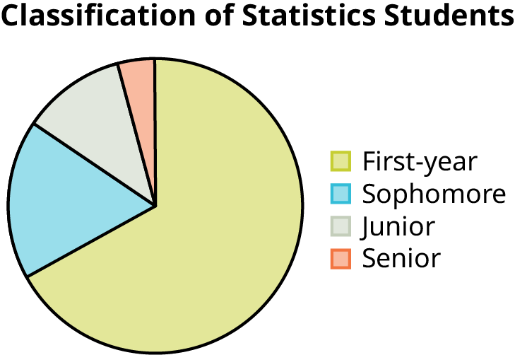
This is a pie chart showing the class classification of statistics students. The chart has 4 sections labeled Freshman, Sophomore, Junior, Senior. A question is asked below the pie chart: what type of data does this graph show?
Figure 1.3 — 1.2 Data, Sampling, and Variation in Data and Sampling

Figure 1.3

Barbara Illowsky and Susan Dean, Introductory Statistics 2E, OpenStax. · CC BY-NC-SA 4.0 · Original image ↗ · Access for free ↗
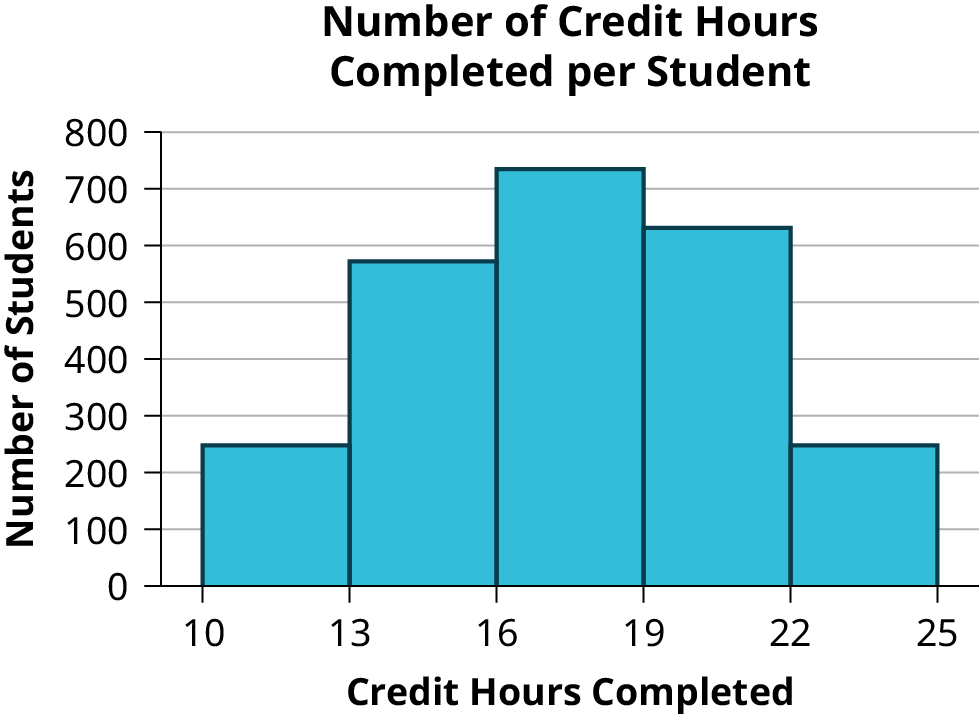
This histogram consists of 5 bars with the x-axis marked at intervals of 3 from 10 to 25, and the y-axis in increments of 100 from 0 to 800. The height of bars shows the number of students in each interval. Interval 10 to 13 is at 250, interval 13 to 16 is at 580, interval 16 to 19 is at 720, interval 19 to 22 is at 620, and interval 22 to 25 is at 250.
Figure 1.4 — 1.2 Data, Sampling, and Variation in Data and Sampling

Figure 1.4

Barbara Illowsky and Susan Dean, Introductory Statistics 2E, OpenStax. · CC BY-NC-SA 4.0 · Original image ↗ · Access for free ↗
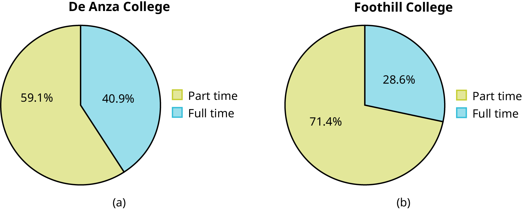
Side-by-side pie charts showing the distribution of part time and full time students. The chart on the left is titled De Anza college. It is divided into two sections showing that part time students represent 59.1% of the population and full time students make up 40.9%. The chart on the right is titled Foothill college. It is divided into two sections showing that part time students represent 71.4% of the population and full time students make up 28.6%.
Figure 1.5 — 1.2 Data, Sampling, and Variation in Data and Sampling

Figure 1.5

Barbara Illowsky and Susan Dean, Introductory Statistics 2E, OpenStax. · CC BY-NC-SA 4.0 · Original image ↗ · Access for free ↗
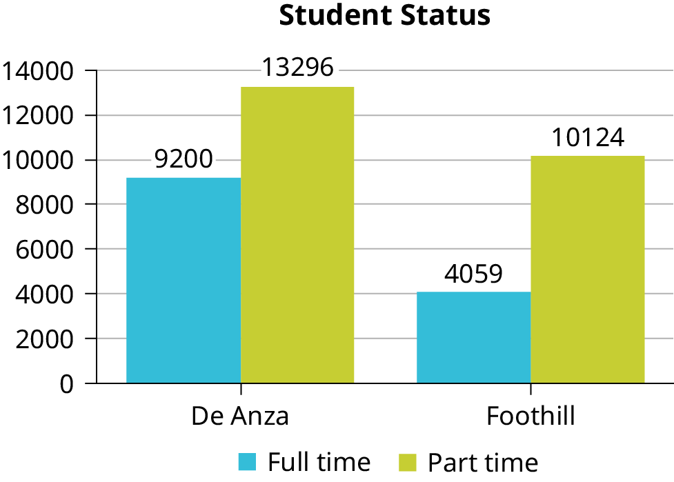
A bar chart titled 'Student Status' shows student numbers for De Anza and Foothill colleges. De Anza has 9,200 full-time and 13,296 part-time students. Foothill has 4,059 full-time and 10,124 part-time students.
Figure 1.6 — 1.2 Data, Sampling, and Variation in Data and Sampling

Figure 1.6

Barbara Illowsky and Susan Dean, Introductory Statistics 2E, OpenStax. · CC BY-NC-SA 4.0 · Original image ↗ · Access for free ↗
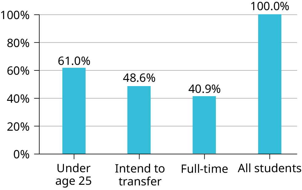
A bar graph. The vertical axis marks values from 0% to 100% in intervals of 20%. The horizontal axis categories are Under age 25 (height of bar shows 61.0%), Intend to transfer (height of bar shows 48.6%), Full-time (height of bar shows 40.9%), and All students (height of bar shows 100%).
Figure 1.7 — 1.2 Data, Sampling, and Variation in Data and Sampling

Figure 1.7

Barbara Illowsky and Susan Dean, Introductory Statistics 2E, OpenStax. · CC BY-NC-SA 4.0 · Original image ↗ · Access for free ↗
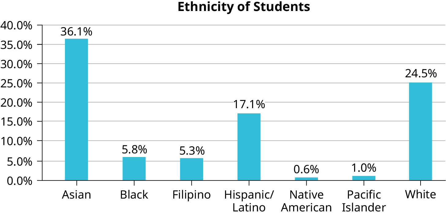
A bar graph showing ethnicity of students. The vertical axis marks values from 0.0% to 40.0% in intervals of 5.0%. The horizontal axis categories are Asian (height of bar shows 36.1%), Black (height of bar shows 5.8%), Filipino (height of bar shows 5.3%), Hispanic/Latino (height of bar shows 17.1%), Native American (height of bar shows 0.6%), Pacific Islander (height of bar shows 1.0%),and White (height of bar shows 24.5%).
Figure 1.8 — 1.2 Data, Sampling, and Variation in Data and Sampling

Figure 1.8

Barbara Illowsky and Susan Dean, Introductory Statistics 2E, OpenStax. · CC BY-NC-SA 4.0 · Original image ↗ · Access for free ↗
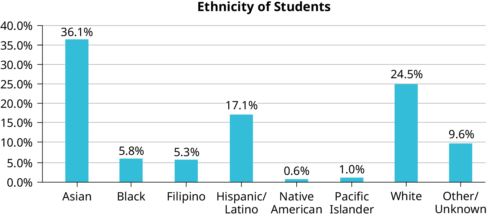
Bar graph consisting of 8 bars with values matching the given data. Horizontal axis has all ethinicity of student. Vertical axis ranges ffrom 0 to 40 percent in increments of 5 percent.
Figure 1.9 — 1.2 Data, Sampling, and Variation in Data and Sampling

Figure 1.9 Bar Graph with Other/Unknown Category

Barbara Illowsky and Susan Dean, Introductory Statistics 2E, OpenStax. · CC BY-NC-SA 4.0 · Original image ↗ · Access for free ↗
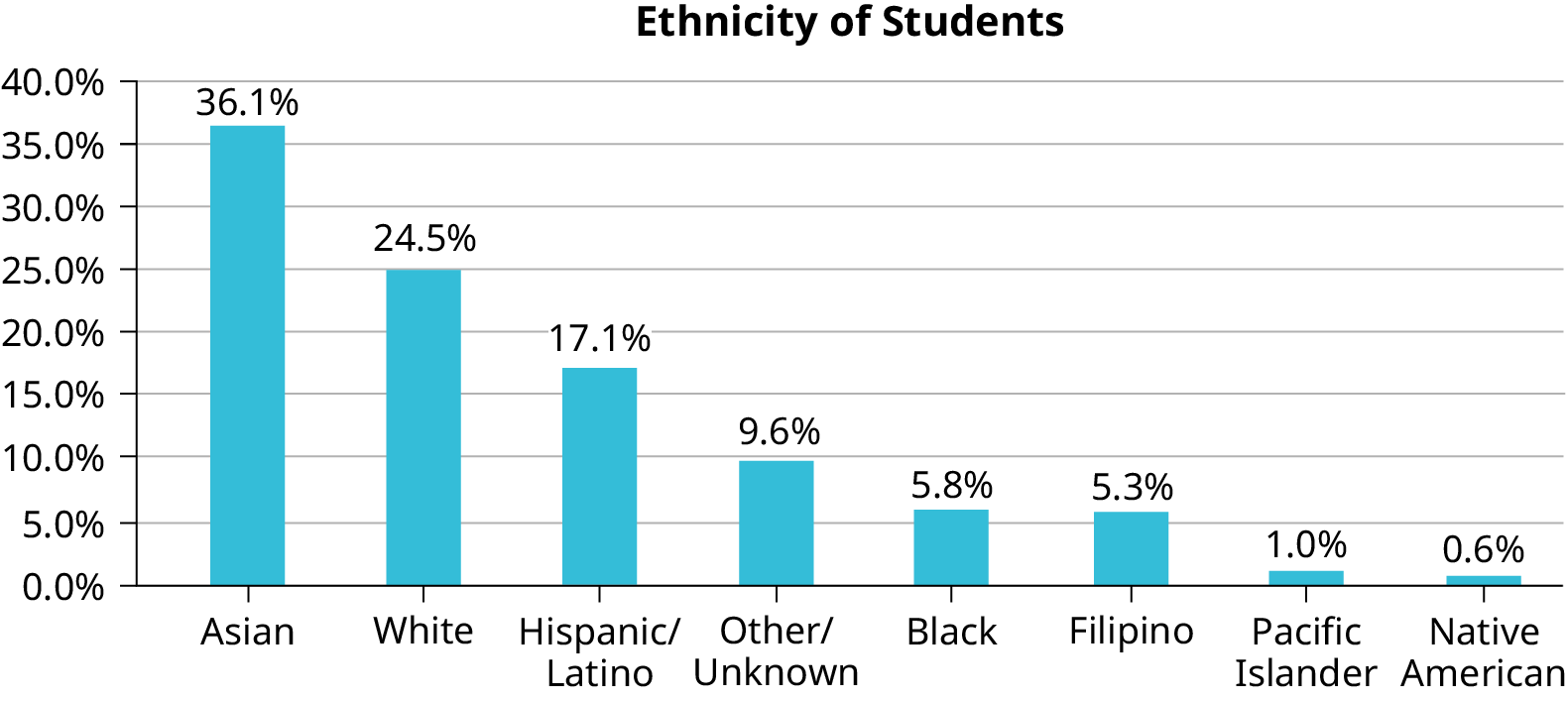
A Pareto chart is a bar graph with the bars ordered from greatest height to least. This one shows ethnicity of students. The vertical axis marks values from 0.0% to 40.0% in intervals of 5.0%. The horizontal axis categories are Asian (height of bar shows 36.1%), White (height of bar shows 24.5%), Hispanic/Latino (height of bar shows 17.1%), Other/Unknown (height of bar shows 9.6%), Black (height of bar shows 5.8%), Filipino (height of bar shows 5.3%), Pacific Islander (height of bar shows 1.0%), and Native American (height of bar shows 0.6%).
Figure 1.10 — 1.2 Data, Sampling, and Variation in Data and Sampling

Figure 1.10 Pareto Chart With Bars Sorted by Size

Barbara Illowsky and Susan Dean, Introductory Statistics 2E, OpenStax. · CC BY-NC-SA 4.0 · Original image ↗ · Access for free ↗
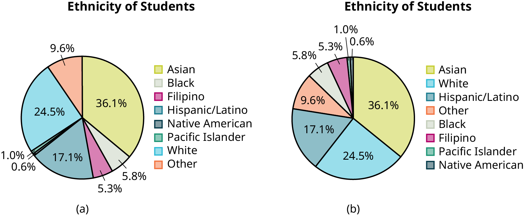
Two pie charts are titled Ethnicity of Students. Chart (a) The sections of the chart are ordered alphabetically. Clockwise from the top, the sections show that Asian students make up 36.1% of students, Black 5.8%, Filipino 5.3%, Hispanic/Latino 17.1%, Native American 0.6%, Pacific Islander 1.0%, White 24.5%, and Other 9.6%. Chart (b) This is the same data as shown in chart (a), but the sections of the chart are now ordered from greatest area to least. Clockwise from the top, the sections show that Asian students make up 36.1% of students, White 24.5%, Hispanic/Latino 17.1%, Other 9.6%, Black 5.8%, Filipino 5.3%, Pacific Islander 1.0%, and Native American 0.6%.
Figure 1.11 — 1.2 Data, Sampling, and Variation in Data and Sampling

Figure 1.11

Barbara Illowsky and Susan Dean, Introductory Statistics 2E, OpenStax. · CC BY-NC-SA 4.0 · Original image ↗ · Access for free ↗
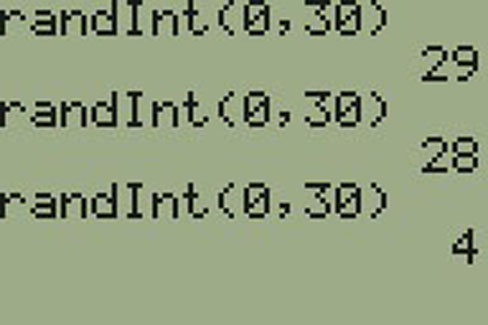
A calculator screen shows the following set on separate lines: randInt (0, 30); 29; randInt (0, 30); 28; randInt (0, 30); 4.
Figure 1.12 — 1.2 Data, Sampling, and Variation in Data and Sampling

Figure 1.12

Barbara Illowsky and Susan Dean, Introductory Statistics 2E, OpenStax. · CC BY-NC-SA 4.0 · Original image ↗ · Access for free ↗
De Anza College Foothill College
Number Percent Number Percent
Full-time 9,200 40.9% Full-time 4,059 28.6%
Part-time 13,296 59.1% Part-time 10,124 71.4%
Total 22,496 100% Total 14,183 100%

Table 1.3 Most Recent Spring Quarter. Barbara Illowsky and Susan Dean, Introductory Statistics 2E, OpenStax.

Characteristic/Category Percent
Full-Time Students 40.9%
Students who intend to transfer to a 4-year educational institution 48.6%
Students under age 25 61.0%
TOTAL 150.5%

Table 1.4 De Anza College Most Recent Spring Quarter. Barbara Illowsky and Susan Dean, Introductory Statistics 2E, OpenStax.

Frequency Percent
Asian 8,794 36.1%
Black 1,412 5.8%
Filipino 1,298 5.3%
Hispanic/Latino 4,180 17.1%
Native American 146 0.6%
Pacific Islander 236 1.0%
White 5,978 24.5%
TOTAL 22,044 out of 24,382 90.4% out of 100%

Table 1.5 Ethnicity of Students at De Anza College in the Most Recent Fall Term. Barbara Illowsky and Susan Dean, Introductory Statistics 2E, OpenStax.

ID Name ID Name ID Name
00 Anselmo 11 King 21 Roquero
01 Bautista 12 Legeny 22 Roth
02 Bayani 13 Lundquist 23 Rowell
03 Cheng 14 Macierz 24 Salangsang
04 Cuarismo 15 Motogawa 25 Slade
05 Cuningham 16 Okimoto 26 Stratcher
06 Fontecha 17 Patel 27 Tallai
07 Hong 18 Price 28 Tran
08 Hoobler 19 Quizon 29 Wai
09 Jiao 20 Reyes 30 Wood
10 Khan

Table 1.6 Class Roster. Barbara Illowsky and Susan Dean, Introductory Statistics 2E, OpenStax.

#1 #2 #3 #4 #5 #6
5 7 10 9 8 3
10 5 9 8 7 6
9 10 8 6 7 9
9 10 10 9 8 9
7 8 9 5 7 4
9 9 9 10 8 7
7 7 10 9 8 8
8 8 9 10 8 8
9 7 8 7 7 8
8 8 10 9 8 7

Table 1.7. Barbara Illowsky and Susan Dean, Introductory Statistics 2E, OpenStax.

Face on Die Frequency
1
2
3
4
5
6

Table 1.8 First Experiment (20 rolls). Barbara Illowsky and Susan Dean, Introductory Statistics 2E, OpenStax.

Face on Die Frequency
1
2
3
4
5
6

Table 1.9 Second Experiment (20 rolls). Barbara Illowsky and Susan Dean, Introductory Statistics 2E, OpenStax.

Source: 1.2 Data, Sampling, and Variation in Data and Sampling

9.4 Rare Events, the Sample, Decision and Conclusion — figures and tables
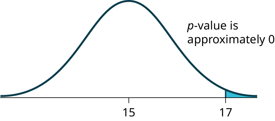
Normal distribution curve on average bread heights with values 15, as the population mean, and 17, as the point to determine the p-value, on the x-axis.
Figure 9.2 — 9.4 Rare Events, the Sample, Decision and Conclusion

Figure 9.2

Barbara Illowsky and Susan Dean, Introductory Statistics 2E, OpenStax. · CC BY-NC-SA 4.0 · Original image ↗ · Access for free ↗

Source: 9.4 Rare Events, the Sample, Decision and Conclusion

3.3 Vector Addition and Subtraction: Analytical Methods — figures and tables
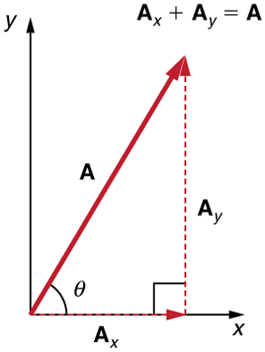
In the given figure a dotted vector A sub x is drawn from the origin along the x axis. From the head of the vector A sub x another vector A sub y is drawn in the upward direction. Their resultant vector A is drawn from the tail of the vector A sub x to the head of the vector A sub y at an angle theta from the x axis. On the graph a vector A, inclined at an angle theta with x axis is shown. Therefore vector A is the sum of the vectors A sub x and A sub y.
Figure 3.24 — 3.3 Vector Addition and Subtraction: Analytical Methods

Figure 3.24 The vector A A , with its tail at the origin of an x , y -coordinate system, is shown together with its x - and y -components, A x A x and A y A y . These vectors form a right triangle. The analytical relationships among these vectors are summarized below.

Paul Peter Urone and Roger Hinrichs, College Physics 2E, OpenStax. · CC BY-NC-SA 4.0 · Original image ↗ · Access for free ↗
]A dotted vector A sub x whose magnitude is equal to A cosine theta is drawn from the origin along the x axis. From the head of the vector A sub x another vector A sub y whose magnitude is equal to A sine theta is drawn in the upward direction. Their resultant vector A is drawn from the tail of the vector A sub x to the head of the vector A-y at an angle theta from the x axis. Therefore vector A is the sum of the vectors A sub x and A sub y.
Figure 3.25 — 3.3 Vector Addition and Subtraction: Analytical Methods

Figure 3.25 The magnitudes of the vector components A x A x and A y A y can be related to the resultant vector A A and the angle θ θ with trigonometric identities. Here we see that A x = A cos θ A x = A cos θ and A y = A sin θ A y = A sin θ .

Paul Peter Urone and Roger Hinrichs, College Physics 2E, OpenStax. · CC BY-NC-SA 4.0 · Original image ↗ · Access for free ↗
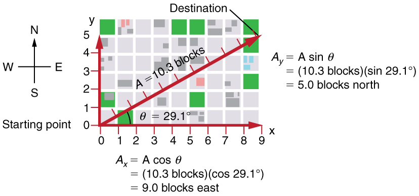
In the given figure a vector A of magnitude ten point three blocks is inclined at an angle twenty nine point one degrees to the positive x axis. The horizontal component A sub x of vector A is equal to A cosine theta which is equal to ten point three blocks multiplied to cosine twenty nine point one degrees which is equal to nine blocks east. Also the vertical component A sub y of vector A is equal to A sin theta is equal to ten point three blocks multiplied to sine twenty nine point one degrees,  which is equal to five point zero blocks north.
Figure 3.26 — 3.3 Vector Addition and Subtraction: Analytical Methods

Figure 3.26 We can use the relationships A x = A cos θ A x = A cos θ and A y = A sin θ A y = A sin θ to determine the magnitude of the horizontal and vertical component vectors in this example.

Paul Peter Urone and Roger Hinrichs, College Physics 2E, OpenStax. · CC BY-NC-SA 4.0 · Original image ↗ · Access for free ↗
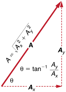
Vector A is shown with its horizontal and vertical components A sub x and A sub y respectively. The magnitude of vector A is equal to the square root of A sub x squared plus A sub y squared. The angle theta of the vector A with the x axis is equal to inverse tangent of A sub y over A sub x
Figure 3.27 — 3.3 Vector Addition and Subtraction: Analytical Methods

Figure 3.27 The magnitude and direction of the resultant vector can be determined once the horizontal and vertical components A x A x and A y A y have been determined.

Paul Peter Urone and Roger Hinrichs, College Physics 2E, OpenStax. · CC BY-NC-SA 4.0 · Original image ↗ · Access for free ↗
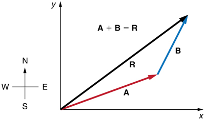
Two vectors A and B are shown. The tail of vector B is at the head of vector A and the tail of the vector A is at origin. Both the vectors are in the first quadrant. The resultant R of these two vectors extending from the tail of vector A to the head of vector B is also shown.
Figure 3.28 — 3.3 Vector Addition and Subtraction: Analytical Methods

Figure 3.28 Vectors A A and B B are two legs of a walk, and R R is the resultant or total displacement. You can use analytical methods to determine the magnitude and direction of R R .

Paul Peter Urone and Roger Hinrichs, College Physics 2E, OpenStax. · CC BY-NC-SA 4.0 · Original image ↗ · Access for free ↗
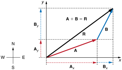
Two vectors A and B are shown. The tail of the vector B is at the head of vector A and the tail of the vector A is at origin. Both the vectors are in the first quadrant. The resultant R of these two vectors extending from the tail of vector A to the head of vector B is also shown. The horizontal and vertical components of the vectors A and B are shown with the help of dotted lines. The vectors labeled as A sub x and A sub y are the components of vector A, and B sub x and B sub y as the components of vector B..
Figure 3.29 — 3.3 Vector Addition and Subtraction: Analytical Methods

Figure 3.29 To add vectors A A and B B , first determine the horizontal and vertical components of each vector. These are the dotted vectors A x A x , A y A y , B x B x and B y B y shown in the image.

Paul Peter Urone and Roger Hinrichs, College Physics 2E, OpenStax. · CC BY-NC-SA 4.0 · Original image ↗ · Access for free ↗
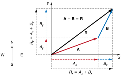
Two vectors A and B are shown. The tail of vector B is at the head of vector A and the tail of the vector A is at origin. Both the vectors are in the first quadrant. The resultant R of these two vectors extending from the tail of vector A to the head of vector B is also shown. The vectors A and B are resolved into the horizontal and vertical components shown as dotted lines parallel to x axis and y axis respectively. The horizontal components of vector A and vector B are labeled as A sub x and B sub x and the horizontal component of the resultant R is labeled at R sub x and is equal to A sub x plus B sub x. The vertical components of vector A and vector B are labeled as A sub y and B sub y and the vertical components of the resultant R is labeled as R sub y is equal to A sub y plus B sub y.
Figure 3.30 — 3.3 Vector Addition and Subtraction: Analytical Methods

Figure 3.30 The magnitude of the vectors A x A x and B x B x add to give the magnitude R x R x of the resultant vector in the horizontal direction. Similarly, the magnitudes of the vectors A y A y and B y B y add to give the magnitude R y R y of the resultant vector in the vertical direction.

Paul Peter Urone and Roger Hinrichs, College Physics 2E, OpenStax. · CC BY-NC-SA 4.0 · Original image ↗ · Access for free ↗
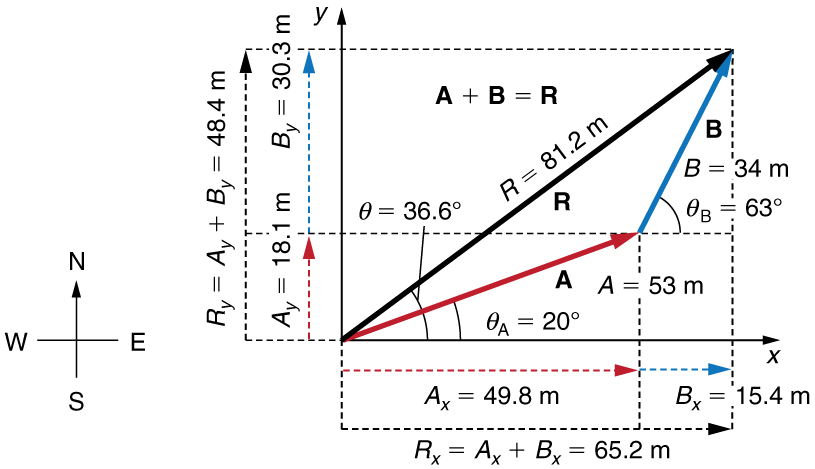
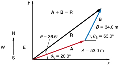
Two vectors A and B are shown. The tail of the vector A is at origin. Both the vectors are in the first quadrant. Vector A is of magnitude fifty three units and is inclined at an angle of twenty degrees to the horizontal. From the head of the vector A another vector B of magnitude 34 units is drawn and is inclined at angle sixty three degrees with the horizontal. The resultant of two vectors is drawn from the tail of the vector A to the head of the vector B.
Figure 3.31 — 3.3 Vector Addition and Subtraction: Analytical Methods

Figure 3.31 Vector A A has magnitude 53 . 0 m 53 . 0 m and direction 20 . 0 º 20 . 0 º north of the x -axis. Vector B B has magnitude 34 . 0 m 34 . 0 m and direction 63 . 0 º 63 . 0 º north of the x -axis. You can use analytical methods to determine the magnitude and direction of R R .

Paul Peter Urone and Roger Hinrichs, College Physics 2E, OpenStax. · CC BY-NC-SA 4.0 · Original image ↗ · Access for free ↗
The addition of two vectors A and B is shown. Vector A is of magnitude fifty three units and is inclined at an angle of twenty degrees to the horizontal. Vector B is of magnitude thirty four units and is inclined at angle sixty three degrees to the horizontal. The components of vector A are shown as dotted vectors A X is equal to forty nine point eight meter along x axis and A Y is equal to eighteen point one meter along Y axis. The components of vector B are also shown as dotted vectors B X is equal to fifteen point four meter and B Y is equal to thirty point three meter. The horizontal component of the resultant R X is equal to A X plus B X is equal to sixty five point two meter. The vertical component of the resultant R Y is equal to A Y plus B Y is equal to forty eight point four meter. The magnitude of the resultant of two vectors is eighty one point two meters. The direction of the resultant R is in thirty six point six degree from the vector A in anticlockwise direction.
Figure 3.32 — 3.3 Vector Addition and Subtraction: Analytical Methods

Figure 3.32 Using analytical methods, we see that the magnitude of R R is 81 . 2 m 81 . 2 m and its direction is 36 . 6º 36 . 6º north of east.

Paul Peter Urone and Roger Hinrichs, College Physics 2E, OpenStax. · CC BY-NC-SA 4.0 · Original image ↗ · Access for free ↗
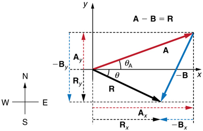
In this figure, the subtraction of two vectors A and B is shown. A red colored vector A is inclined at an angle theta A to the positive of x axis. From the head of vector A a blue vector negative B is drawn. Vector B is in west of south direction. The resultant of the vector A and vector negative B is shown as a black vector R from the tail of vector A to the head of vector negative B. The resultant R is inclined to x axis at an angle theta below the x axis. The components of the vectors are also shown along the coordinate axes as dotted lines of their respective colors.
Figure 3.33 — 3.3 Vector Addition and Subtraction: Analytical Methods

Figure 3.33 The subtraction of the two vectors shown in Figure 3.28 . The components of –B –B are the negatives of the components of B B . The method of subtraction is the same as that for addition.

Paul Peter Urone and Roger Hinrichs, College Physics 2E, OpenStax. · CC BY-NC-SA 4.0 · Original image ↗ · Access for free ↗

Source: 3.3 Vector Addition and Subtraction: Analytical Methods

1.2 Physical Quantities and Units — figures and tables
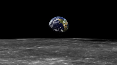
A view of Earth from the Moon.
Figure 1.15 — 1.2 Physical Quantities and Units

Figure 1.15 The distance from Earth to the Moon may seem immense, but it is just a tiny fraction of the distances from Earth to other celestial bodies. (credit: NASA)

Paul Peter Urone and Roger Hinrichs, College Physics 2E, OpenStax. (credit: NASA) · CC BY-NC-SA 4.0 · Original image ↗ · Access for free ↗
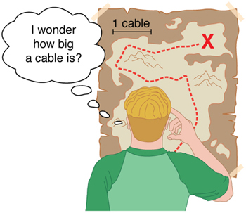
A boy looking at a map and trying to guess distances with unit of length mentioned as cables between two points.
Figure 1.16 — 1.2 Physical Quantities and Units

Figure 1.16 Distances given in unknown units are maddeningly useless.

Paul Peter Urone and Roger Hinrichs, College Physics 2E, OpenStax. · CC BY-NC-SA 4.0 · Original image ↗ · Access for free ↗
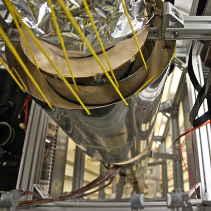
A top view of an atomic fountain is shown. It measures time using the vibration of the cesium atom.
Figure 1.17 — 1.2 Physical Quantities and Units

Figure 1.17 An atomic clock such as this one uses the vibrations of cesium atoms to keep time to a precision of better than a microsecond per year. The fundamental unit of time, the second, is based on such clocks. This image is looking down from the top of an atomic fountain nearly 30 feet tall! (credit: Steve Jurvetson/Flickr)

Paul Peter Urone and Roger Hinrichs, College Physics 2E, OpenStax. (credit: Steve Jurvetson/Flickr) · CC BY-NC-SA 4.0 · Original image ↗ · Access for free ↗
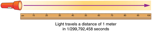
Beam of light from a flashlight is represented by an arrow pointing right, traveling the length of a meter stick.
Figure 1.18 — 1.2 Physical Quantities and Units

Figure 1.18 The meter is defined to be the distance light travels in 1/299,792,458 of a second in a vacuum. Distance traveled is speed multiplied by time.

Paul Peter Urone and Roger Hinrichs, College Physics 2E, OpenStax. · CC BY-NC-SA 4.0 · Original image ↗ · Access for free ↗
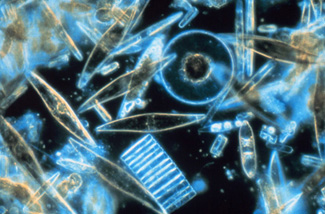
A magnified image of tiny phytoplankton swimming among the crystal of ice.[
Figure 1.19 — 1.2 Physical Quantities and Units

Figure 1.19 Tiny phytoplankton swims among crystals of ice in the Antarctic Sea. They range from a few micrometers to as much as 2 millimeters in length. (credit: Prof. Gordon T. Taylor, Stony Brook University; NOAA Corps Collections)

Paul Peter Urone and Roger Hinrichs, College Physics 2E, OpenStax. (credit: Prof. Gordon T. Taylor, Stony Brook University; NOAA Corps Collections) · CC BY-NC-SA 4.0 · Original image ↗ · Access for free ↗
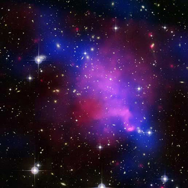
A view of Abell Galaxy with some bright stars and some hot gases.
Figure 1.20 — 1.2 Physical Quantities and Units

Figure 1.20 Galaxies collide 2.4 billion light years away from Earth. The tremendous range of observable phenomena in nature challenges the imagination. (credit: NASA/CXC/UVic./A. Mahdavi et al. Optical/lensing: CFHT/UVic./H. Hoekstra et al.)

Paul Peter Urone and Roger Hinrichs, College Physics 2E, OpenStax. (credit: NASA/CXC/UVic./A. Mahdavi et al. Optical/lensing: CFHT/UVic./H. Hoekstra et al.) · CC BY-NC-SA 4.0 · Original image ↗ · Access for free ↗
Length Mass Time
meter (m) kilogram (kg) second (s) ampere (A)

Table 1.1 Fundamental SI Units. Paul Peter Urone and Roger Hinrichs, College Physics 2E, OpenStax.

Prefix Symbol Value Example (some are approximate)
exa E 10 18 exameter Em 10 18  m distance light travels in a century
peta P 10 15 petasecond Ps 10 15  s 30 million years
tera T 10 12 terawatt TW 10 12  W powerful laser output
giga G 10 9 gigahertz GHz 10 9  Hz a microwave frequency
mega M 10 6 megacurie MCi 10 6  Ci high radioactivity
kilo k 10 3 kilometer km 10 3  m about 6/10 mile
hecto h 10 2 hectoliter hL 10 2  L 26 gallons
deka da 10 1 dekagram 10 1  g teaspoon of butter
— — 100 (=1)
deci d 10 − 1 deciliter dL 10 − 1  L less than half a soda
centi c 10 − 2 10 − 2  m fingertip thickness
milli m 10 − 3 millimeter mm 10 − 3  m flea at its shoulders
micro µ 10 − 6 micrometer 10 − 6  m detail in microscope
nano n 10 − 9 nanogram ng 10 − 9  g small speck of dust
pico p 10 − 12 picofarad pF 10 − 12  F small in radio
femto f 10 − 15 femtometer fm 10 − 15  m size of a
atto a 10 − 18 attosecond as 10 − 18  s time light crosses an

Table 1.2 Metric Prefixes for Powers of 10 and their Symbols. Paul Peter Urone and Roger Hinrichs, College Physics 2E, OpenStax.

Lengths in meters Masses in kilograms (more precise values in parentheses) Times in seconds (more precise values in parentheses)
10 − 18 Present experimental limit to smallest observable detail 10 − 30 Mass of an 9.11×10⁻³¹ kg 10 − 23 Time for light to cross a
10 − 15 Diameter of a 10 − 27 Mass of a hydrogen 1.67×10⁻²⁷ kg 10 − 22 Mean life of an extremely unstable
10 − 14 Diameter of a uranium 10 − 15 Mass of a 10 − 15 Time for one oscillation of visible light
10 − 10 Diameter of a hydrogen 10 − 5 Mass of a mosquito 10 − 13 Time for one vibration of an in a solid
10 − 8 Thickness of in cells of living organisms 10 − 2 Mass of a hummingbird 10 − 8 Time for one oscillation of an FM radio wave
10 − 6 of visible light 1 Mass of a liter of water (about a quart) 10 − 3 Duration of a nerve impulse
10 − 3 Size of a grain of sand 10 2 Mass of a person 1 Time for one heartbeat
1 Height of a 4-year-old child 10 3 Mass of a car 10 5 One day 8.64×10⁴s
10 2 Length of a football field 10 8 Mass of a large ship 10 7 One year (y) 3.16×10⁷s
10 4 Greatest ocean depth 10 12 Mass of a large iceberg 10 9 About half the life expectancy of a human
10 7 Diameter of the Earth 10 15 Mass of the of a comet 10 11 Recorded history
10 11 Distance from the Earth to the Sun 10 23 Mass of the Moon 7.35×10²² kg 10 17 Age of the Earth
10 16 Distance traveled by light in 1 year (a light year) 10 25 Mass of the Earth 5.97×1024 kg 10 18 Age of the universe
10 21 Diameter of the Milky Way galaxy 10 30 Mass of the Sun 1.99×1030 kg
10 22 Distance from the Earth to the nearest large galaxy (Andromeda) 10 42 Mass of the Milky Way galaxy (current upper limit)
10 26 Distance from the Earth to the edges of the known universe 10 53 Mass of the known universe (current upper limit)

Table 1.3 Approximate Values of Length, Mass, and Time. Paul Peter Urone and Roger Hinrichs, College Physics 2E, OpenStax.
Source: 1.2 Physical Quantities and Units

190 terms, alphabetically ordered

Acid · ·

In the Brønsted–Lowry model, a substance that can donate a . Acidic have a higher activity than water.

Read explanation · OpenStax ↗
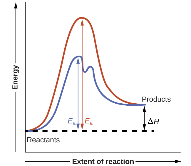
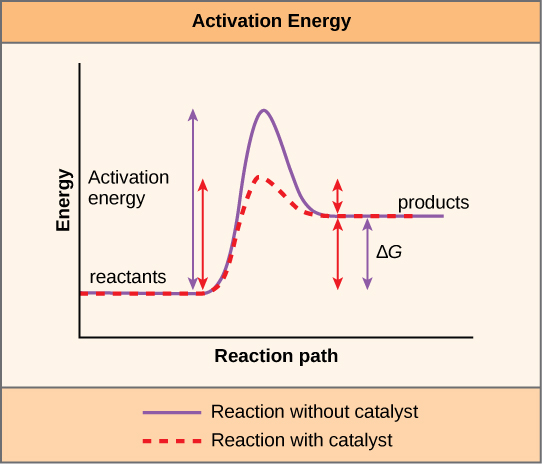
Activation energy ·

The energy barrier that must overcome to reach a and undergo .

Read explanation · OpenStax ↗
Active catalytic-site concentration ·

The total of active sites used to calculate from . It equals active when each has one site.

Read explanation · Biology LibreTexts ↗
Active site

The region of an that binds its and carries out .

Read explanation · OpenStax ↗
Adenosine triphosphate

An energy-carrying ; its powers many cellular processes, including cycles.

Read explanation · OpenStax ↗
Alpha carbon · ·

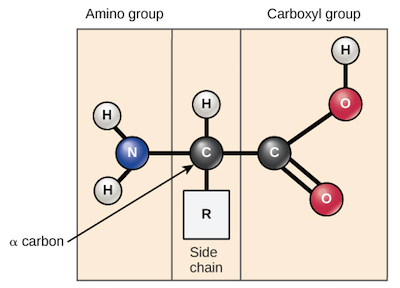
The central carbon next to the carboxyl carbon. In a standard it binds an , hydrogen, and .

Read explanation · OpenStax ↗
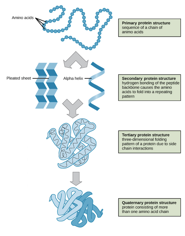
Alpha helix · · · · · ·

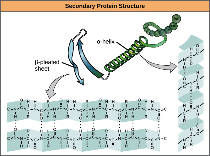
A helical stabilized by between a oxygen and an hydrogen four later.

Read explanation · OpenStax ↗
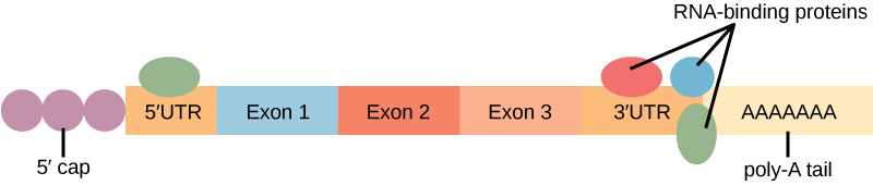
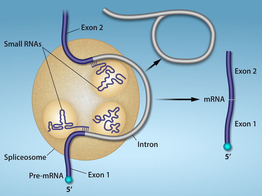
Alternative splicing ·

Regulated or context-dependent use of different or combinations to generate different mature from one precursor.

Read explanation · OpenStax ↗
Amide · · ·

A group containing a carbon bonded to nitrogen. are amide linkages.

Read explanation · OpenStax ↗
Amino acid

A building block containing amino and and a characteristic .

Read explanation · OpenStax ↗
Amino acid residue · ·

The part of an incorporated into a chain. Residue can also describe another building block within a larger .

Read explanation · OpenStax ↗
Amino group · · ·

A nitrogen-containing . A free ’s amino group is typically (NH₃⁺) near physiological ; ’s ring nitrogen is an exception to this formula.

Read explanation · OpenStax ↗
Amphipathic

Having both a region and a region, as in a or .

Read explanation · OpenStax ↗
Analytical standard ·

A material with a known identity or amount used to compare or calibrate measurements.

Read explanation · Agilent ↗
Anticodon

A triplet that pairs to an . The anticodon for 5′-AUG-3′ is aligned 3′-UAC-5′, or written 5′-CAU-3′.

Read explanation · NCBI Bookshelf / Garland Science ↗
Antiparallel

Running in opposite directions, as with two strands or neighboring strands in some .

Read explanation · OpenStax ↗
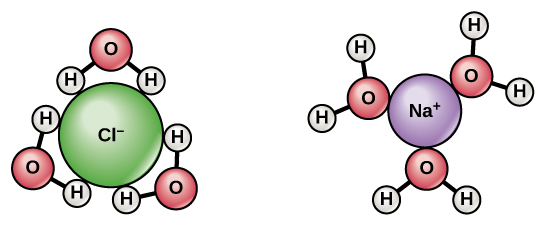
Aqueous solution ·

A in which water is the .

Read explanation · OpenStax ↗
Archaea ·

A of distinct from , with characteristic chemistry and -expression machinery.

Read explanation · OpenStax ↗
Aromatic

Containing a cyclic, with . , , and have aromatic .

Read explanation · OpenStax ↗
Atom

The smallest unit of an element that retains its chemical identity; it has a surrounded by .

Read explanation · OpenStax ↗
Bacteria ·

A of single-celled . Bacterial cells lack a -bound and are distinct from .

Read explanation · OpenStax ↗
Benzene ring

A six-carbon ring with .

Read explanation · OpenStax ↗
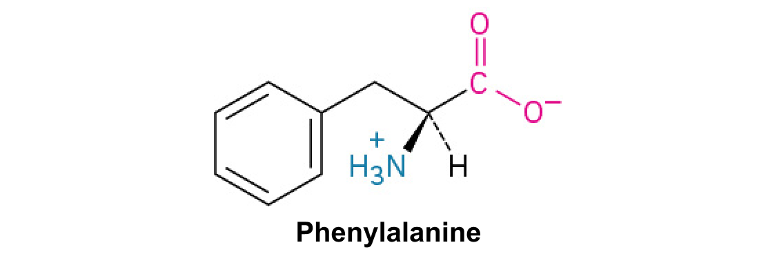
Benzyl group

A attached through a –CH₂– group; part of ’s .

Read explanation · OpenStax ↗
Beta sheet · · · · · ·

A made of aligned segments connected by ; strands may be parallel or .

Read explanation · OpenStax ↗
Biomolecule

A made by or involved in living systems, including , , , and .

Read explanation · OpenStax ↗
Blotting ·

Transfer of separated or to a so a specific target can be detected.

Read explanation · Thermo Fisher ↗
Brønsted–Lowry base · · · · · · · · · · ·

In the Brønsted–Lowry model, a substance that can accept a . Basic solutions have lower activity than water.

Read explanation · OpenStax ↗
Calibration

Establishing the relation between a measured signal and known values or .

Read explanation · Agilent ↗
Cancer

A group of diseases involving abnormal cells that can proliferate without normal restraints and invade tissues.

Read explanation · OpenStax ↗
capacitor

Device storing separated and electric-field energy.

Read explanation · OpenStax ↗
Carbohydrate

A class of including sugars and their , used for energy storage, structure, and recognition.

Read explanation · OpenStax ↗
Carbonyl group · ·

A carbon double-bonded to oxygen, C=O; present in and many other .

Read explanation · OpenStax ↗
Carboxyl group · ·

An , COOH. In free it is usually to COO⁻ near physiological .

Read explanation · OpenStax ↗
Catalyst · ·

A substance that speeds a by providing a pathway with lower and is regenerated rather than consumed overall.

Read explanation · OpenStax ↗
Catalytic efficiency · ·

The ratio kcat/Km, describing performance at low . Units are ⁻¹ time⁻¹, commonly M⁻¹ s⁻¹.

Read explanation · IUBMB ↗
Centimeter

A unit of length equal to one hundredth of a meter.

Read explanation · NIST ↗
Chemical reaction ·

A process that rearranges and chemical bonds, converting into .

Read explanation · OpenStax ↗
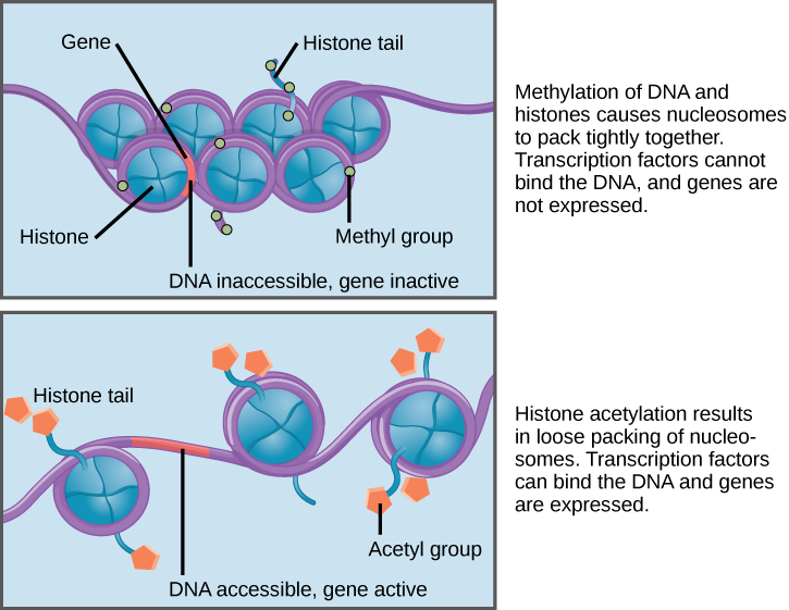
Chromatin

The complex of and associated , including , in .

Read explanation · OpenStax ↗
Chromatography

Separation of mixture components by their different interactions with a and a moving .

Read explanation · Waters ↗
Chromosome ·

An organized with associated that carries . A replicated chromosome has two .

Read explanation · OpenStax ↗
Codon

A sequence of three that specifies an or a stop signal.

Read explanation · OpenStax ↗
complement

A system that can promote , , and attack against targets.

Read explanation · OpenStax ↗
Concentration

The amount of a substance in a specified volume or mass of mixture.

Read explanation · OpenStax ↗
Conjugated system ·

Adjacent orbitals that allow to be distributed across several , often through alternating single and multiple bonds.

Read explanation · OpenStax ↗
convenience sample

A sample selected because its members are readily accessible rather than through a population-based probability scheme.

Read explanation · OpenStax ↗
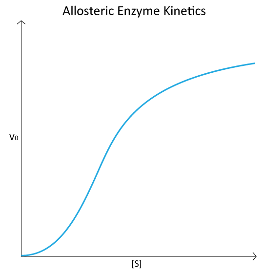
Cooperativity · ·

An interaction in which binding at one site changes binding at other sites. Positive cooperativity can produce a response.

Read explanation · Biology LibreTexts ↗
Covalent bond · ·

A bond in which share pairs. and are covalent.

Read explanation · OpenStax ↗
Cysteine ·

An with a . Two cysteines can form a .

Read explanation · OpenStax ↗
DAG

Diacylglycerol, a -associated messenger that helps activate .

Read explanation · OpenStax ↗
Deoxyribonucleic acid

The that stores genetic information used to specify and sequences.

Read explanation · OpenStax ↗
Deprotonation

Removal of a from a or group; this changes its by minus one.

Read explanation · OpenStax ↗
Detergent

An substance that can associate with both water and material; detergents can disrupt or interactions.

Read explanation · Thermo Fisher ↗
determination

Developmental commitment to a cell fate before all specialized features necessarily appear.

Read explanation · OpenStax ↗
dimensional analysis

Checking or relating expressions by their underlying units such as length, mass, and time.

Read explanation · OpenStax ↗
Disulfide bond · · ·

A covalent sulfur–sulfur bond formed by of two , which can stabilize structure.

Read explanation · NCBI Bookshelf ↗
DNA replication

Copying so genetic information can be passed to daughter cells. Each guides a complementary new strand.

Read explanation · OpenStax ↗
Electric charge · · ·

An electrical property that can be positive or negative. Opposite charges attract and like charges repel; net charge is the sum of all charges on a particle.

Read explanation · OpenStax ↗
electric current

Rate of flow through a cross section, measured in amperes.

Read explanation · OpenStax ↗
Electric field

A quantity describing the electrical force per unit positive . An applied field drives through a gel during .

Read explanation · Thermo Fisher ↗
Electron

A negatively subatomic particle. Electron sharing and transfer determine much of chemical bonding.

Read explanation · OpenStax ↗
Electron delocalization ·

Distribution of across several rather than confinement to one or bond.

Read explanation · OpenStax ↗
Electronegativity ·

An ’s tendency to attract shared in a chemical bond. Unequal attraction can make a bond .

Read explanation · OpenStax ↗
Electrophoresis

Movement of in an , used to separate through a support such as a gel.

Read explanation · Thermo Fisher ↗
Enzyme

A biological that speeds a without being consumed. Most enzymes are .

Read explanation · OpenStax ↗
Enzyme saturation · ·

The high- limit in which sites spend almost all their time processing and the rate approaches .

Read explanation · Biology LibreTexts ↗
ethnicity

Shared cultural history, ancestry, language, or affiliation.

Read explanation · OpenStax ↗
Eukaryote ·

An organism whose cells have a -enclosed ; animals, plants, fungi, and protists are eukaryotes.

Read explanation · OpenStax ↗
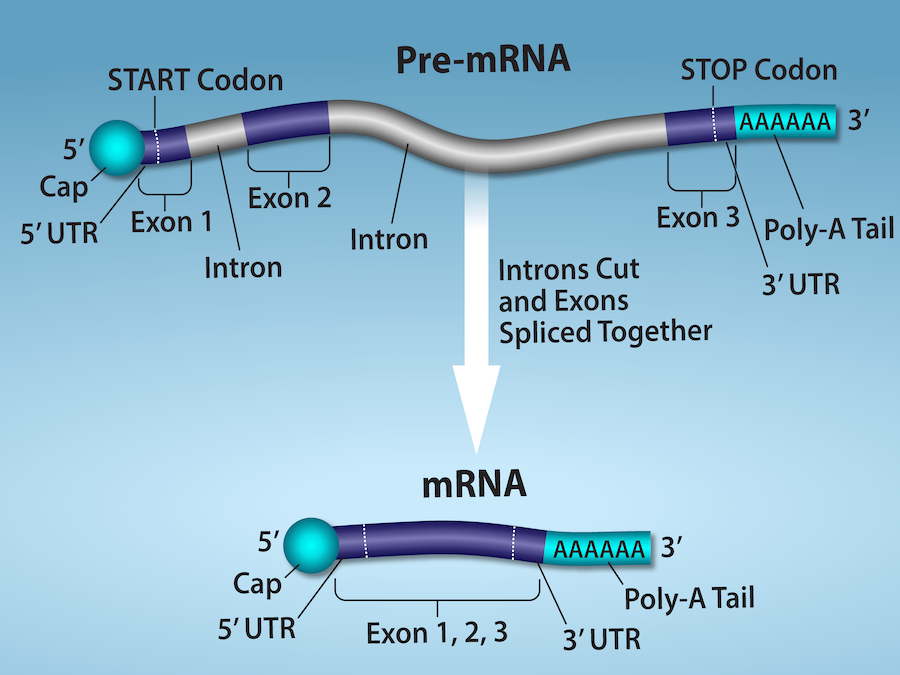
Exon

A segment retained in a mature spliced . In an exon may contain coding sequence, untranslated sequence, or both.

Read explanation · OpenStax ↗
FACT complex ·

A -associated complex that helps machinery traverse and supports reorganization.

Read explanation · OpenStax ↗
First-order kinetics

A rate dependence proportional to the first power of a . At low , a is approximately first-order in .

Read explanation · Biology LibreTexts ↗
Fraction · ·

A portion of a sample collected during a separation, such as the fluid leaving a column during a time interval.

Read explanation · Waters ↗
Functional group

A group of whose chemical behavior gives a characteristic and properties.

Read explanation · OpenStax ↗
Gene

A sequence that contributes to a functional or , together with the information needed to express it.

Read explanation · OpenStax ↗
Gene expression

Production of a functional from a , including and, for -coding , .

Read explanation · NCBI Bookshelf ↗
Half-life

The time required for half of a population or amount to remain during decay; a constant half-life is characteristic of decay.

Read explanation · OpenStax ↗
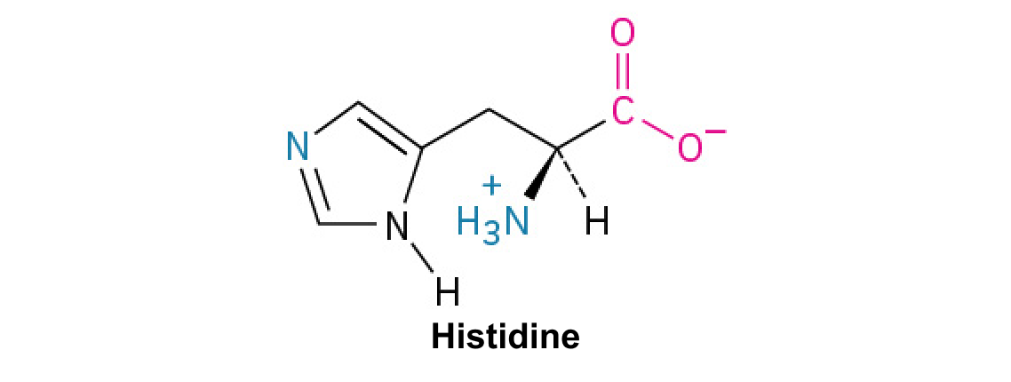
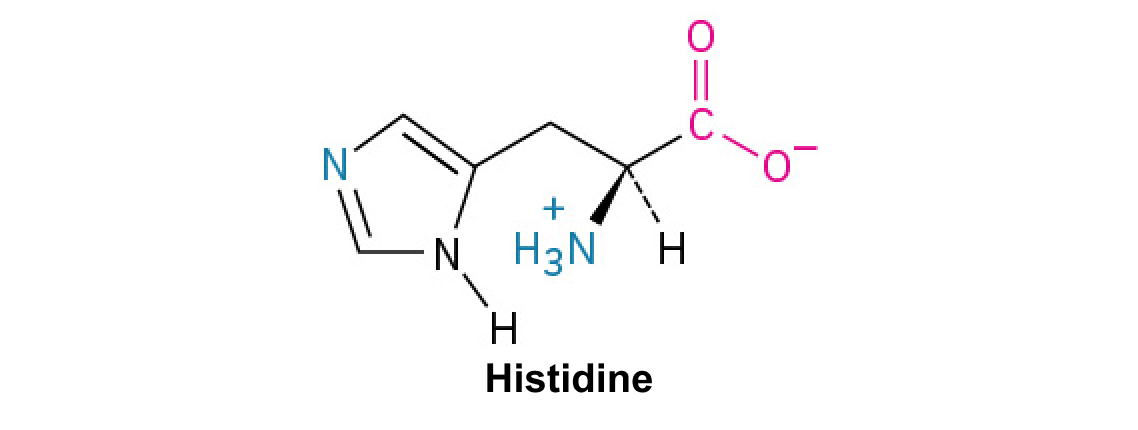
Histidine ·

A with an . Mostly uncharged near physiological , it can accept or donate .

Read explanation · OpenStax ↗
Histone

A -associated rich in . Core histones form the around which nucleosomal wraps.

Read explanation · OpenStax ↗
Histone acetyltransferase · ·

An adding acetyl groups to lysines, often promoting accessible and .

Read explanation · OpenStax ↗
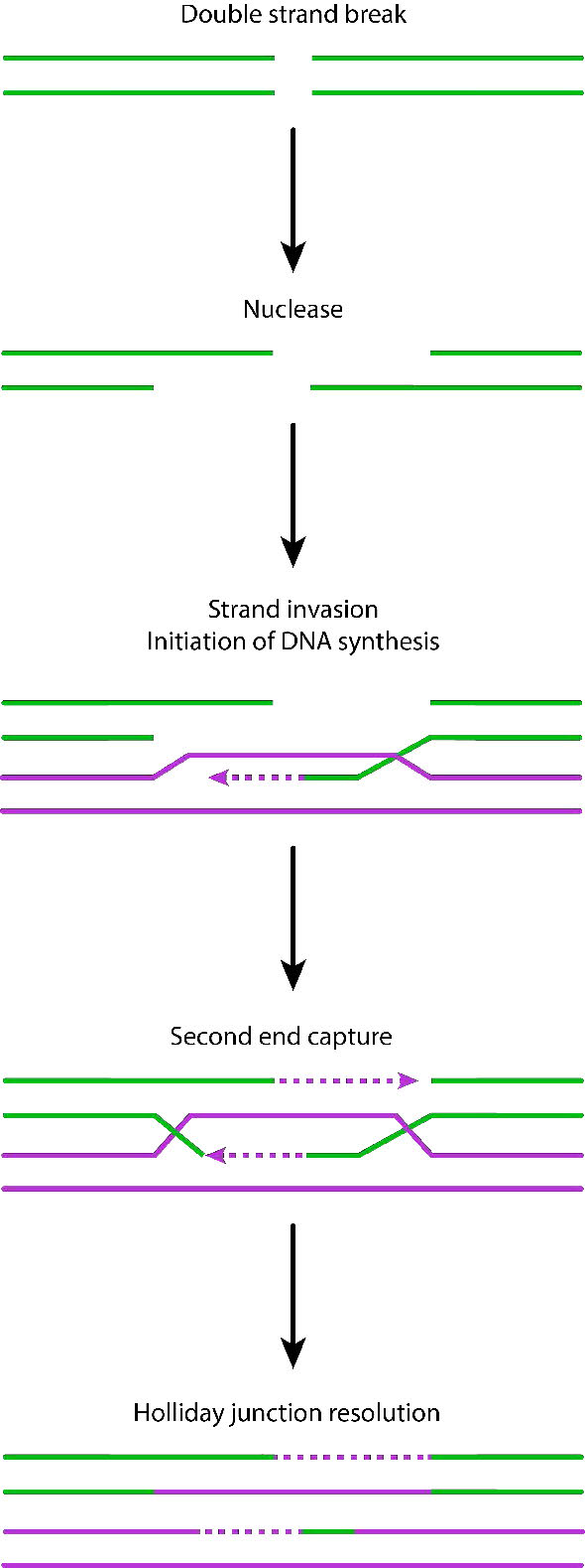
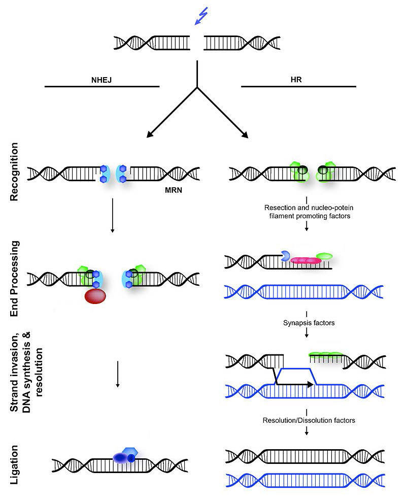
Homologous recombination ·

Exchange or copying between with similar sequences. In break repair, an intact homologous template, usually a , guides restoration.

Read explanation · Biology LibreTexts / Oregon State University ↗
Hydrogen bond ·

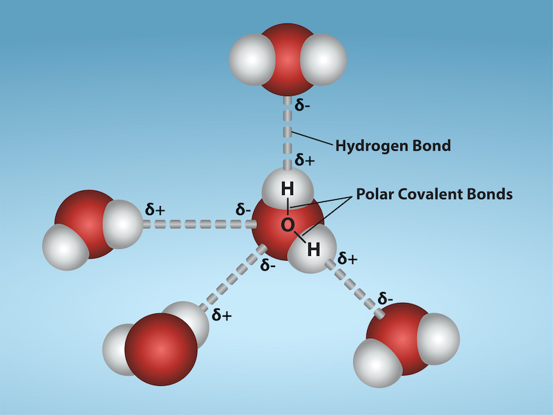
An attraction between a hydrogen bonded to an and another . hydrogen bonds stabilize .

Read explanation · OpenStax ↗
Hydrogen ion · ·

A positively hydrogen species. H⁺ denotes a , which is hydrated in water; its activity determines .

Read explanation · OpenStax ↗
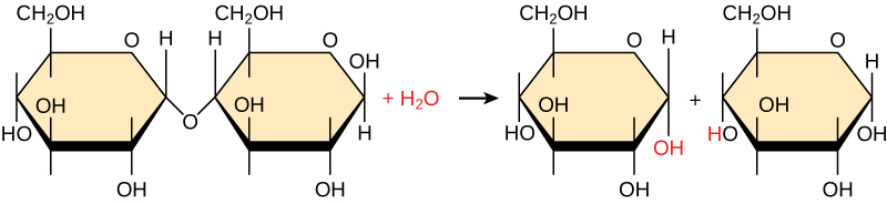
Hydrolysis

Breaking a chemical bond by adding water. hydrolysis separates .

Read explanation · OpenStax ↗
Hydrophilic

Interacting favorably with water, typically because a group is or .

Read explanation · OpenStax ↗
Hydrophobic

Interacting poorly with water. often gather in a ’s interior.

Read explanation · OpenStax ↗
Hydroxide ion ·

The negatively OH⁻. Basic contain a higher hydroxide ion activity than water at the same temperature.

Read explanation · OpenStax ↗
Hydroxyl group ·

An oxygen bonded to hydrogen, –OH. Hydroxyl groups can and often increase .

Read explanation · OpenStax ↗
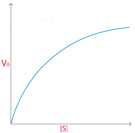
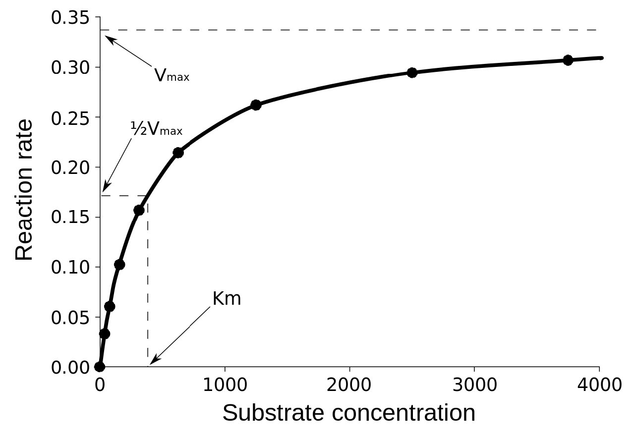
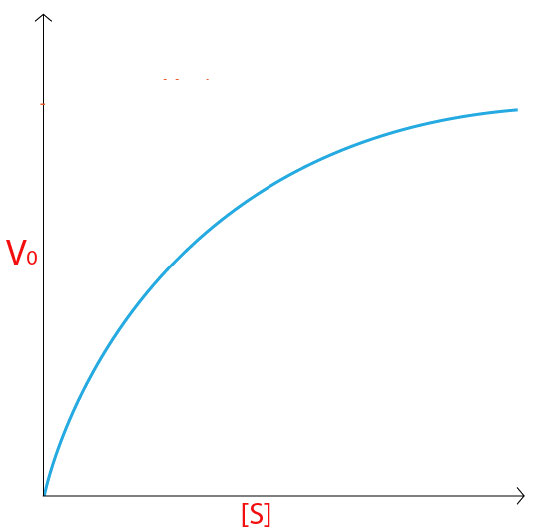
Hyperbolic curve ·

A curve that approaches an asymptote. The standard rate curve is a rectangular hyperbola approaching .

Read explanation · Biology LibreTexts ↗
Imidazole

A five-membered ring containing two nitrogens; ’s contains this ring.

Read explanation · OpenStax ↗
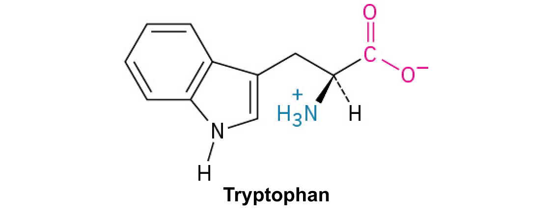
Indole

A fused six-membered and five-membered ring system containing nitrogen; found in .

Read explanation · OpenStax ↗
inflammation

A coordinated tissue response recruiting defense and repair mechanisms, often involving increased blood flow and permeability.

Read explanation · OpenStax ↗
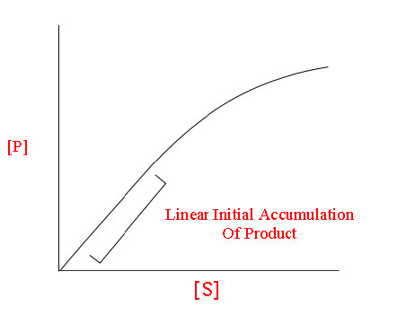
Initial reaction rate · · · ·

The early rate of formation, measured before substantial depletion or accumulation, usually after the brief binding transient.

Read explanation · Biology LibreTexts ↗
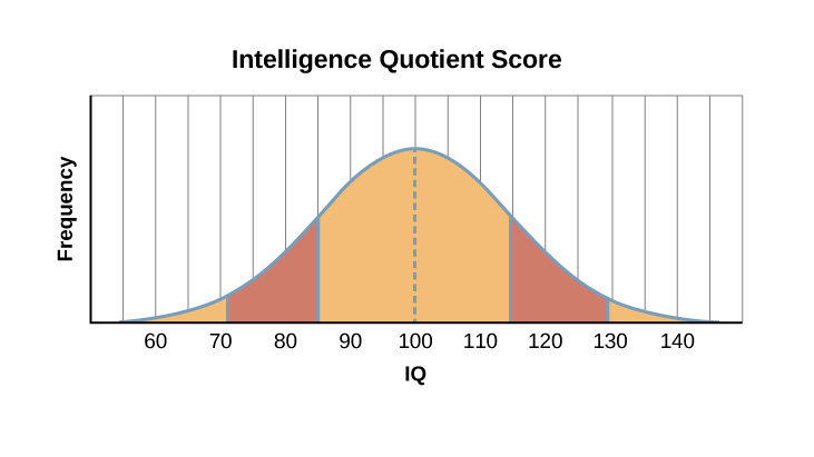
intelligence quotient

Standardized score comparing cognitive-test performance with a .

Read explanation · OpenStax ↗
Intron ·

A segment removed from a precursor during . Intronic signals or regulatory sequences can affect .

Read explanation · OpenStax ↗
Ion · ·

An or with a net because its numbers of and do not balance.

Read explanation · OpenStax ↗
Isoform

One of several related or forms produced from a , for example through .

Read explanation · OpenStax ↗
Kinase ·

An that transfers a , often from , to a target .

Read explanation · Thermo Fisher ↗
kinematics

Description of motion without specifying its causes.

Read explanation · OpenStax ↗
linkage

A tendency of nearby on the same to be inherited together.

Read explanation · OpenStax ↗
Lipid

A broad class of largely or , including fats, , and steroids.

Read explanation · OpenStax ↗
locus

The specific position of a or other feature.

Read explanation · OpenStax ↗
Logarithm · · ·

The exponent needed to obtain a number from a chosen fixed number. For decimal logarithms, log₁₀(100) = 2 because 10² = 100; uses the negative decimal logarithm of activity.

Read explanation · OpenStax ↗
Matrix

A supporting material, such as a gel or the solid support in a column. Its properties influence movement and binding of sample .

Read explanation · Thermo Fisher ↗
Maximum reaction rate · ·

The limiting as becomes saturating. For a fixed under given conditions, Vmax = times .

Read explanation · Biology LibreTexts ↗
Membrane · · · ·

A thin boundary or sheet. Cell membranes are bilayers containing ; membranes are synthetic supports that hold or for detection.

Read explanation · OpenStax ↗
Messenger RNA ·

An that carries coding information used by to synthesize a .

Read explanation · OpenStax ↗
Michaelis–Menten kinetics · ·

A model with = [S]/(Km + ). Its curve is ; may require a different model.

Read explanation · Biology LibreTexts ↗
Micromolar ·

A of 10⁻⁶ moles per liter. Convert micromolar to molar when expressing in M⁻¹ s⁻¹.

Read explanation · NIST ↗
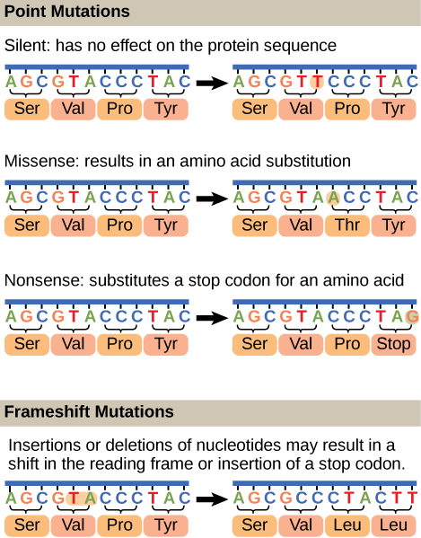
Missense mutation ·

A coding-sequence that changes the specified ; its effect depends on the and context.

Read explanation · OpenStax ↗
Mobile phase

The moving fluid that carries a sample through a system.

Read explanation · Waters ↗
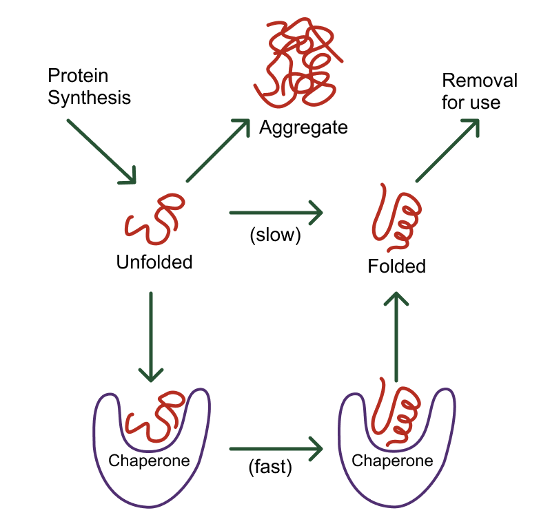
Molecular chaperone · ·

A that assists other in folding or prevents , without specifying their sequence.

Read explanation · NCBI Bookshelf ↗
Molecule

Two or more joined by . A molecule may be electrically or carry a .

Read explanation · OpenStax ↗
Mutation

A change in a sequence; some mutations alter a ’s sequence.

Read explanation · OpenStax ↗
Native structure · · ·

A ’s functional folded arrangement under its normal conditions.

Read explanation · NCBI Bookshelf ↗
Neutral

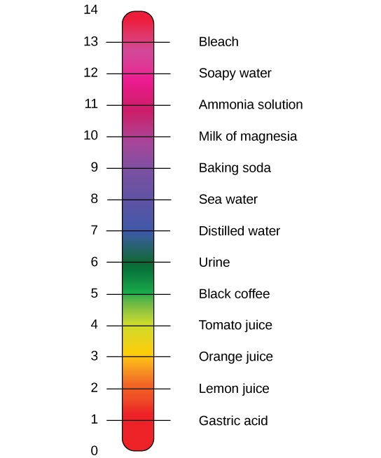
Having no net . For a , neutral instead means equal and activities; its is about 7 at 25 °C.

Read explanation · OpenStax ↗
Nitrogenous base · · ·

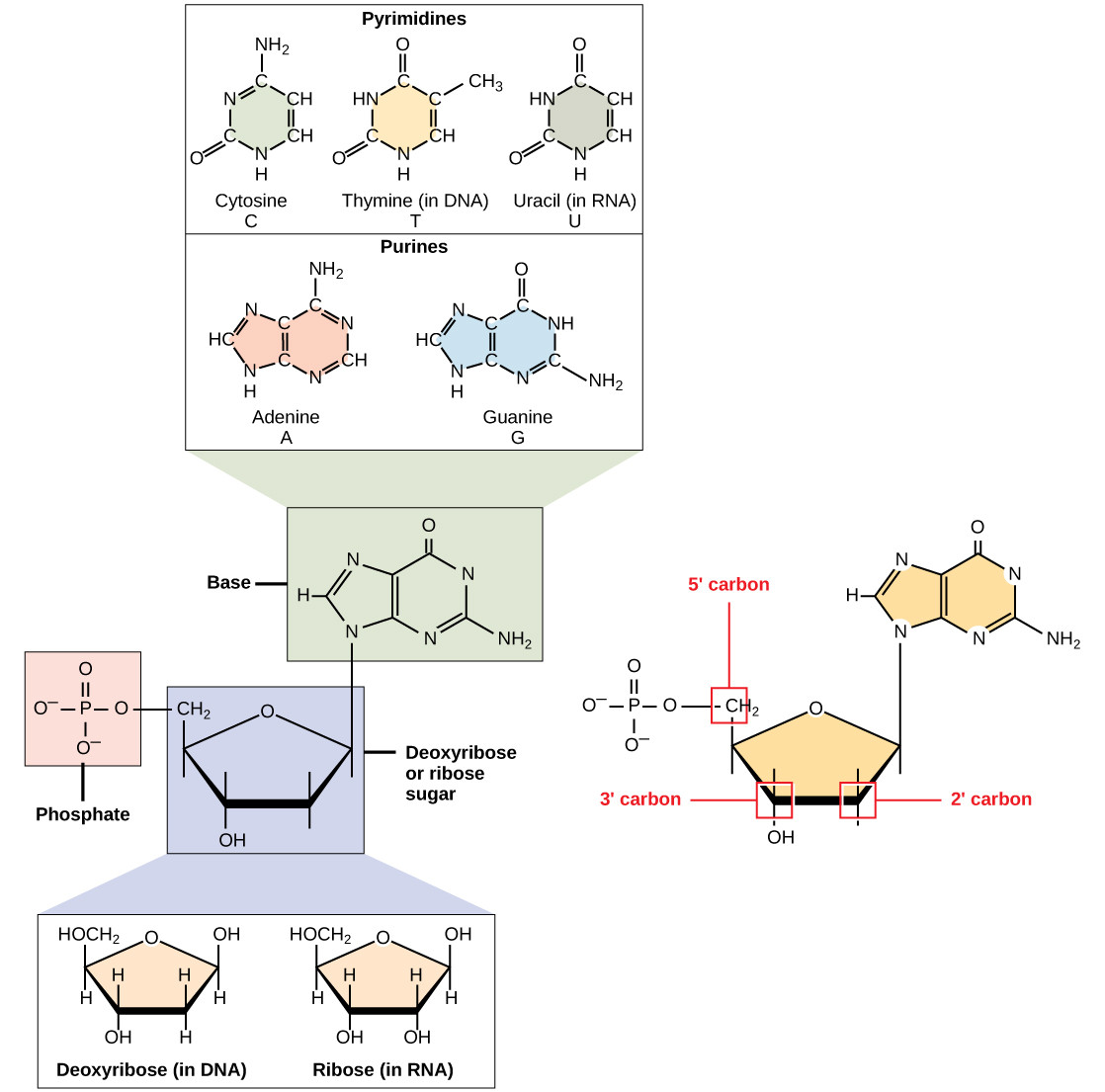
A nitrogen-containing ring component of ; its pairing interactions help specify sequences.

Read explanation · OpenStax ↗
Nonpolar ·

Lacking a substantial separation of . Nonpolar groups generally interact poorly with water.

Read explanation · OpenStax ↗
Nonsense mutation ·

A that converts an amino- into a premature , potentially truncating the or destabilizing its .

Read explanation · OpenStax ↗
Nucleic acid

A of , such as or , used in information storage, expression, and other cellular functions.

Read explanation · OpenStax ↗
Nucleosome

The basic unit of : wrapped around a .

Read explanation · OpenStax ↗
Nucleotide

A joined to a sugar and one or more .

Read explanation · OpenStax ↗
Nucleus ·

A -enclosed compartment containing most of a cell’s .

Read explanation · OpenStax ↗
null hypothesis

A specified population model or parameter claim against which observed data are evaluated.

Read explanation · OpenStax ↗
Octamer

A complex made of eight . A core contains eight .

Read explanation · OpenStax ↗
opsonization

Coating a target with that enhance its recognition and uptake by phagocytes.

Read explanation · OpenStax ↗
Oxidation ·

Loss of or an increase in oxidation state. Oxidizing two can form a .

Read explanation · OpenStax ↗
Peptide

A chain of joined by ; the term commonly describes chains shorter than a typical .

Read explanation · OpenStax ↗
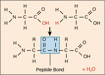
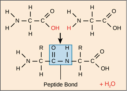
Peptide bond ·

A covalent between the carboxyl carbon of one and the amino nitrogen of the next.

Read explanation · OpenStax ↗
pH

A measure of , defined as the negative of activity. Lower pH means greater ; pH influences .

Read explanation · OpenStax ↗
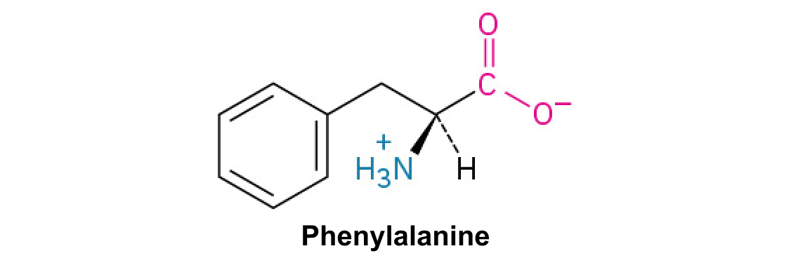
Phenylalanine ·

A with an .

Read explanation · OpenStax ↗
Phosphate group ·

A phosphorus-containing group bonded to oxygens; phosphate groups occur in , , and modified .

Read explanation · OpenStax ↗
Phospholipid

An with a -containing region and tails; a major component of cellular .

Read explanation · OpenStax ↗
photon

Quantum of electromagnetic radiation with energy hf.

Read explanation · OpenStax ↗
PKC

Protein kinase C, a family regulated by signals and, for conventional , calcium.

Read explanation · OpenStax ↗
Polar

Having an uneven distribution of . Polar groups often interact favorably with water.

Read explanation · OpenStax ↗
Polyacrylamide

A used to form a gel for separating by .

Read explanation · Thermo Fisher ↗
Polyacrylamide gel electrophoresis ·

Electrophoretic separation using a . Native PAGE preserves much of a ’s .

Read explanation · Thermo Fisher ↗
Polymer

A large made from many linked molecular building blocks.

Read explanation · OpenStax ↗
Polypeptide

A chain of connected by . A functional can contain one or several such chains.

Read explanation · OpenStax ↗
Porous material · · · ·

A material containing small spaces that can admit of suitable size.

Read explanation · Cytiva ↗
Prokaryote ·

An organism whose cells lack a -bound ; and are prokaryotes.

Read explanation · OpenStax ↗
Proline ·

An whose loops back to the nitrogen, restricting rotation and often creating bends.

Read explanation · OpenStax ↗
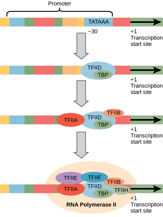
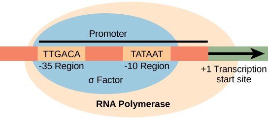
Promoter

A region that recruits machinery and helps specify where and in which direction begins.

Read explanation · OpenStax ↗
Protein

One or more folded chains that perform biological roles such as , transport, signaling, or structural support.

Read explanation · OpenStax ↗
Protein aggregation · ·

Association of into larger clusters, often when exposed surfaces of unfolded stick together.

Read explanation · NCBI Bookshelf ↗
Protein backbone ·

The repeating nitrogen–alpha-carbon– chain of a , excluding its variable .

Read explanation · OpenStax ↗
Protein domain · ·

A region of a that forms a recognizable structural or functional unit.

Read explanation · OpenStax ↗
Proton

A positively subatomic particle. In – chemistry, donating a proton means transferring a .

Read explanation · OpenStax ↗
Protonation

Addition of a to an , , or ; this changes its by plus one.

Read explanation · OpenStax ↗
Qualitative analysis

Analysis that identifies a substance or property without necessarily measuring its amount.

Read explanation · Agilent ↗
Quantification · ·

Estimating the amount or of a substance from measured signals and suitable or .

Read explanation · Waters ↗
R group · ·

The variable side chain attached to an ’s . It determines identity, , , and chemical behavior.

Read explanation · OpenStax ↗
Reactant

A starting substance transformed during a .

Read explanation · OpenStax ↗
Reaction intermediate · ·

A species formed in one step and consumed in another. It occupies a local energy minimum between .

Read explanation · OpenStax ↗
Reaction product ·

A substance formed by a .

Read explanation · OpenStax ↗
reaction quotient

-to- activity ratio with stoichiometric exponents at the current composition.

Read explanation · OpenStax ↗
Reaction rate · ·

How quickly are consumed or form, usually expressed as a change per unit time.

Read explanation · OpenStax ↗
reference group

Group used as a standard for evaluation or comparison.

Read explanation · OpenStax ↗
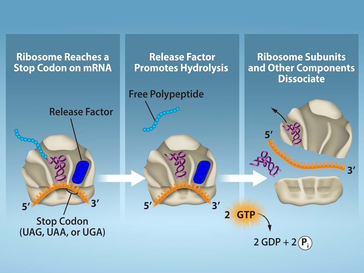
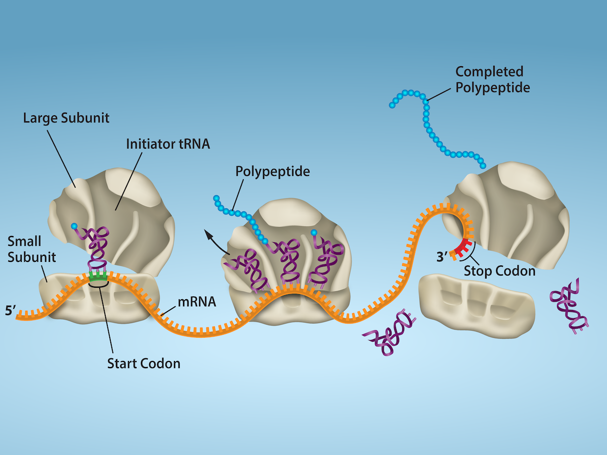
Release factor ·

A that recognizes a stop signal and promotes of the – to release the .

Read explanation · OpenStax ↗
Ribonucleic acid ·

A with roles in , regulation, and ; carries -coding information.

Read explanation · OpenStax ↗
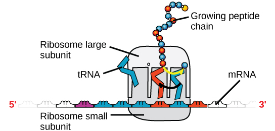
Ribosome ·

A complex of and that translates into a .

Read explanation · OpenStax ↗
RNA splicing · ·

Removal of and joining of in a precursor .

Read explanation · NCBI Bookshelf / Garland Science ↗
RNA stability

Persistence of an before degradation; greater stability generally means a longer lifetime or under specified conditions.

Read explanation · OpenStax ↗
sampling bias

Systematic distortion arising when the selected sample differs from the intended population in relevant ways.

Read explanation · OpenStax ↗
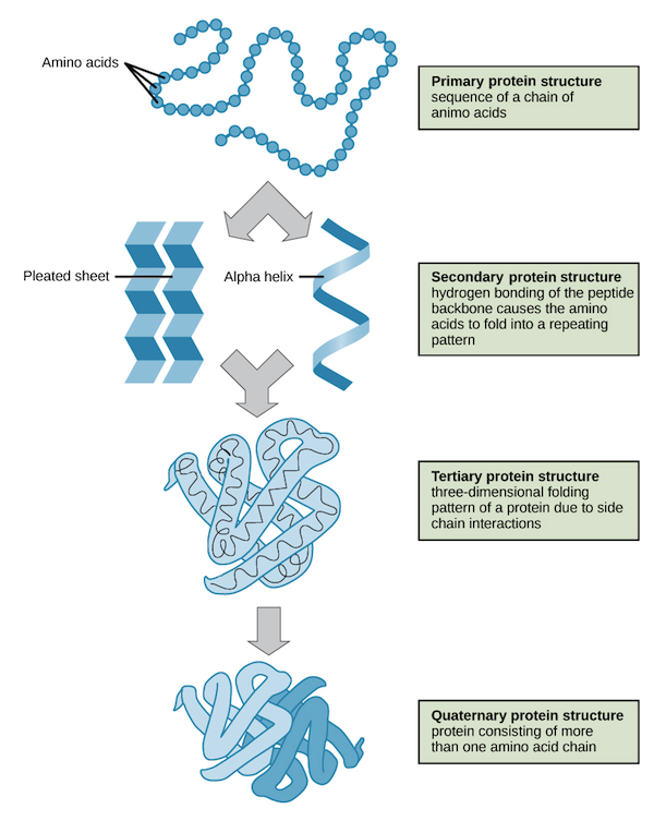
Secondary structure

Local folding, such as and , stabilized mainly by .

Read explanation · OpenStax ↗
Sigma factor · · ·

A -polymerase-associated factor that helps recognize sequences and initiate .

Read explanation · OpenStax ↗
Sigmoidal curve ·

An S-shaped curve. A sigmoidal rate-versus- curve can indicate rather than simple behavior.

Read explanation · Biology LibreTexts ↗
Sister chromatid

One of the two copies of a produced by . An intact sister chromatid can supply a template for accurate repair.

Read explanation · Biology LibreTexts / Oregon State University ↗
Solubility ·

The amount of a substance that can dissolve in a under specified conditions. Soluble means able to dissolve; insoluble means only very slightly soluble in that .

Read explanation · OpenStax ↗
Solute

A dissolved component of a .

Read explanation · OpenStax ↗
Solution

A homogeneous mixture in which are dissolved in a .

Read explanation · OpenStax ↗
Solvent

The component of a that dissolves other substances, usually the component present in the greatest amount.

Read explanation · OpenStax ↗
Splice site · · ·

A sequence at an – boundary recognized during ; changing it can alter use or removal.

Read explanation · OpenStax ↗
standard deviation

A measure of dispersion around a mean expressed in the original variable’s units.

Read explanation · OpenStax ↗
Stationary phase

The material that remains fixed in a system.

Read explanation · Waters ↗
Stop codon · · ·

An that recruits a to end : UAA, UAG, or UGA in the standard code.

Read explanation · OpenStax ↗
Substitution · ·

Replacement of one by another. In a coding region it can be , , or .

Read explanation · OpenStax ↗
Substrate

A that an binds and chemically transforms.

Read explanation · OpenStax ↗
Substrate concentration

The amount of per volume. Square brackets denote ; [S] is varied to measure an curve.

Read explanation · Biology LibreTexts ↗
Subunit ·

An individual chain within a containing multiple chains.

Read explanation · OpenStax ↗
Synonymous mutation · · · · ·

A coding-sequence that leaves the specified unchanged. It can still affect , , or .

Read explanation · OpenStax ↗
Template strand · · ·

A preexisting strand whose sequence guides complementary nucleic- synthesis.

Read explanation · OpenStax ↗
Thiol group · · · ·

A sulfur bonded to hydrogen, –SH. thiols can form through .

Read explanation · OpenStax ↗
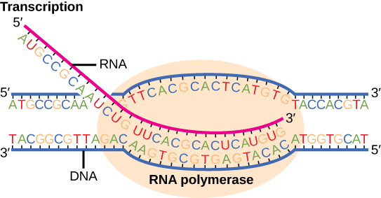
Transcription

Synthesis of using a template.

Read explanation · OpenStax ↗
Transfer RNA ·

An adaptor that carries an and pairs its with a on .

Read explanation · OpenStax ↗
Transition state

A fleeting, high-energy arrangement at a barrier. It is an energy maximum along the path, rather than a stable .

Read explanation · OpenStax ↗
Translation ·

Synthesis of a on a using the sequence of in .

Read explanation · OpenStax ↗
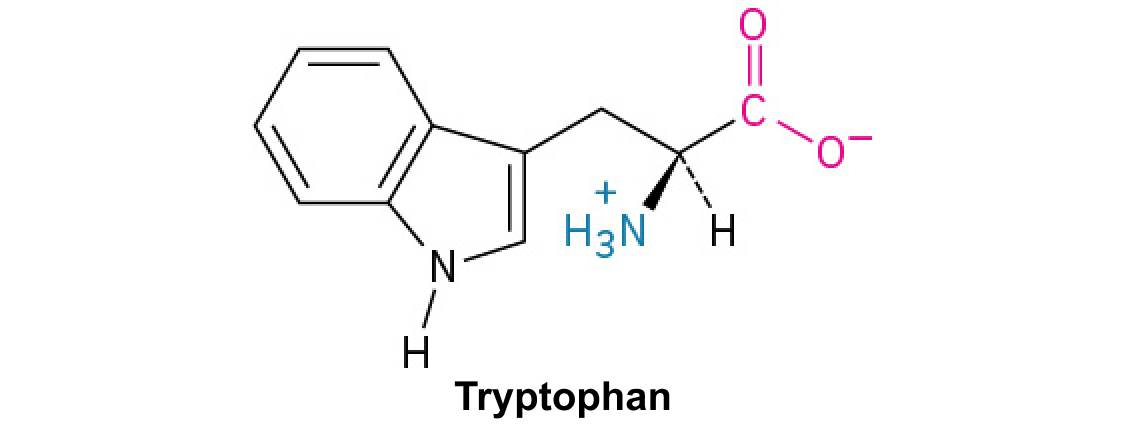
Tryptophan ·

An with a bulky ; commonly grouped as .

Read explanation · OpenStax ↗
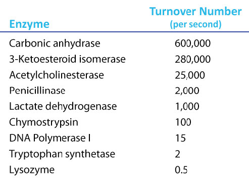
Turnover number · · ·

The maximum number of cycles per per unit time, calculated as /. Units are inverse time, commonly s⁻¹.

Read explanation · IUBMB ↗
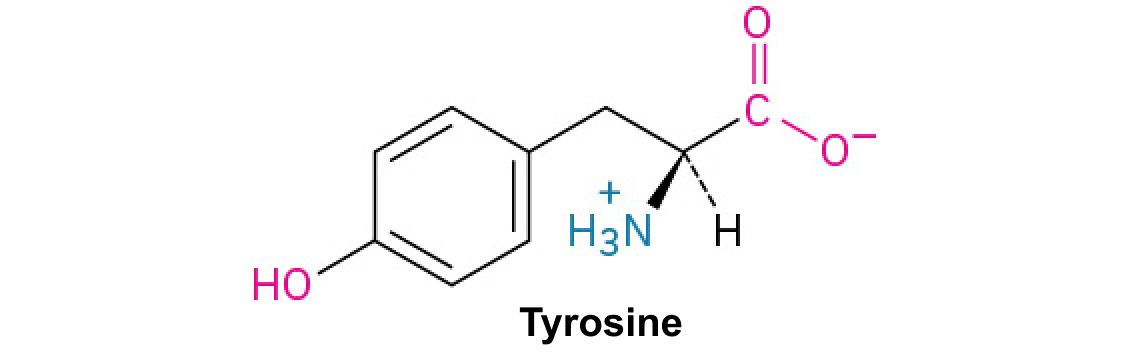
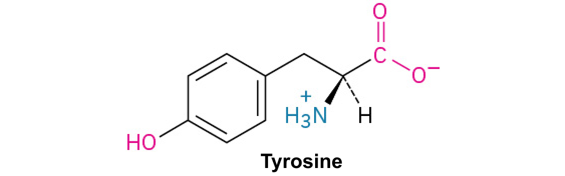
Tyrosine ·

An with a phenolic . Usually uncharged near physiological .

Read explanation · OpenStax ↗
Wavelength

The distance between repeating points of a wave, such as neighboring crests; light wavelength determines energy.

Read explanation · JASCO ↗

1.2 Data, Sampling, and Variation in Data and Sampling

OpenStax · 1.2 Data, Sampling, and Variation in Data and Sampling ↗
Instructional page including learning objectives, examples, figures, source tables and questions. Site navigation and embedded media players are omitted; source media links remain available.

Data may come from a population or from a sample. Lowercase letters like x or y generally are used to represent data values. Most data can be put into the following categories:

data are the result of categorizing or describing attributes of a population. data are also often called categorical data. Hair color, blood type, ethnic group, the car a person drives, and the street a person lives on are examples of data. data are generally described by words or letters. For instance, hair color might be black, dark brown, light brown, blonde, gray, or red. Blood type might be AB+, O-, or B+. Researchers often prefer to use data over data because it lends itself more easily to mathematical analysis. For example, it does not make sense to find an average hair color or blood type.

data are always numbers. data are the result of counting or measuring attributes of a population. Amount of money, pulse rate, weight, number of people living in your town, and number of students who take statistics are examples of data. data may be either discrete or continuous.

All data that are the result of counting are called discrete data. These data take on only certain numerical values. If you count the number of phone calls you receive for each day of the week, you might get values such as zero, one, two, or three.

Data that are not only made up of counting numbers, but that may include , decimals, or irrational numbers, are called continuous data. Continuous data are often the results of measurements like lengths, weights, or times. A list of the lengths in minutes for all the phone calls that you make in a week, with numbers like 2.4, 7.5, or 11.0, would be continuous data.

Example 1.5

Data Sample of Discrete Data

The data are the number of books students carry in their backpacks. You sample five students. Two students carry three books, one student carries four books, one student carries two books, and one student carries one book. The numbers of books (three, four, two, and one) are the discrete data.

Try It 1.5

The data are the number of machines in a gym. You sample five gyms. One gym has 12 machines, one gym has 15 machines, one gym has ten machines, one gym has 22 machines, and the other gym has 20 machines. What type of data is this?

Example 1.6

Data Sample of Continuous Data

The data are the weights of backpacks with books in them. You sample the same five students. The weights (in pounds) of their backpacks are 6.2, 7, 6.8, 9.1, 4.3. Notice that backpacks carrying three books can have different weights. Weights are continuous data.

Try It 1.6

The data are the areas of lawns in square feet. You sample five houses. The areas of the lawns are 144 sq. feet, 160 sq. feet, 190 sq. feet, 180 sq. feet, and 210 sq. feet. What type of data is this?

Example 1.7

You go to the supermarket and purchase three cans of soup (19 ounces tomato bisque, 14.1 ounces lentil, and 19 ounces Italian wedding), two packages of nuts (walnuts and peanuts), four different kinds of vegetable (broccoli, cauliflower, spinach, and carrots), and two desserts (16 ounces pistachio ice cream and 32 ounces chocolate chip cookies).

Problem

Name data sets that are discrete, continuous, and .

One Possible :

  • The three cans of soup, two packages of nuts, four kinds of vegetables and two desserts are discrete data because you count them.
  • The weights of the soups (19 ounces, 14.1 ounces, 19 ounces) are continuous data because you measure weights as precisely as possible.
  • Types of soups, nuts, vegetables and desserts are data because they are categorical.

Try to identify additional data sets in this example.

Try It 1.7

The following list of materials was purchased by a purchase manager in a company:

  • Two types of nails (2 kg box nails, 3 kg roofing nails)
  • One type of oil (4 L machine oil)
  • Four types of screws (3 kg wood screws, 5 kg machine screws, 1 kg set screws, 2 kg socket screws)

Name data sets that are discrete, continuous, and .

Example 1.8

The data are the colors of backpacks. Again, you sample the same five students. One student has a red backpack, two students have black backpacks, one student has a green backpack, and one student has a gray backpack. The colors red, black, black, green, and gray are data.

Try It 1.8

The data are the colors of houses. You sample five houses. The colors of the houses are white, yellow, white, red, and white. What type of data is this?

NOTE

You may collect data as numbers and report it categorically. For example, the quiz scores for each student are recorded throughout the term. At the end of the term, the quiz scores are reported as A, B, C, D, or F.

Example 1.9

Problem

Work collaboratively to determine the correct data type ( or ). Indicate whether data are continuous or discrete. Hint: Data that are discrete often start with the words "the number of."

  1. the number of pairs of shoes you own
  2. the type of car you drive
  3. the distance it is from your home to the nearest grocery store
  4. the number of classes you take per school year.
  5. the type of calculator you use
  6. weights of dogs at an animal shelter
  7. number of correct answers on a quiz
  8. scores (This may cause some discussion.)

Items a, d, and g are discrete; items c, f, and h are continuous; items b and e are , or categorical.

Try It 1.9

Determine the correct data type ( or ) for the number of cars in a parking lot. Indicate whether data are continuous or discrete.

Example 1.10

Problem

A statistics professor collects information about the classification of her students as first-year students, sophomores, juniors, or seniors. The data she collects are summarized in the pie chart Figure 1.3. What type of data does this graph show?

This is a pie chart showing the class classification of statistics students. The chart has 4 sections labeled Freshman, Sophomore, Junior, Senior. A question is asked below the pie chart: what type of data does this graph show?
Figure 1.3 — 1.2 Data, Sampling, and Variation in Data and Sampling

Figure 1.3

Barbara Illowsky and Susan Dean, Introductory Statistics 2E, OpenStax. · CC BY-NC-SA 4.0 · Original image ↗ · Access for free ↗

This pie chart shows the students in each year, which is (or categorical) data.

Try It 1.10

The registrar at State University keeps records of the number of credit hours students complete each semester. The data collected are summarized in the histogram. The class boundaries are 10 to less than 13, 13 to less than 16, 16 to less than 19, 19 to less than 22, and 22 to less than 25.

This histogram consists of 5 bars with the x-axis marked at intervals of 3 from 10 to 25, and the y-axis in increments of 100 from 0 to 800. The height of bars shows the number of students in each interval. Interval 10 to 13 is at 250, interval 13 to 16 is at 580, interval 16 to 19 is at 720, interval 19 to 22 is at 620, and interval 22 to 25 is at 250.
Figure 1.4 — 1.2 Data, Sampling, and Variation in Data and Sampling

Figure 1.4

Barbara Illowsky and Susan Dean, Introductory Statistics 2E, OpenStax. · CC BY-NC-SA 4.0 · Original image ↗ · Access for free ↗


What type of data does this graph show?

Data Discussion

Below are tables comparing the number of part-time and full-time students at De Anza College and Foothill College enrolled for the most recent spring quarter. The tables display counts (frequencies) and percentages or proportions (relative frequencies). The percent columns make comparing the same categories in the colleges easier. Displaying percentages along with the numbers is often helpful, but it is particularly important when comparing sets of data that do not have the same totals, such as the total enrollments for both colleges in this example. Notice how much larger the percentage for part-time students at Foothill College is compared to De Anza College.

De Anza College Foothill College
Number Percent Number Percent
Full-time 9,200 40.9% Full-time 4,059 28.6%
Part-time 13,296 59.1% Part-time 10,124 71.4%
Total 22,496 100% Total 14,183 100%
Table 1.3 Most Recent Spring Quarter

Tables are a good way of organizing and displaying data. But graphs can be even more helpful in understanding the data. There are no strict rules concerning which graphs to use. Two graphs that are used to display data are pie charts and bar graphs.

In a pie chart, categories of data are represented by wedges in a circle and are proportional in size to the percent of individuals in each category.

In a bar graph, the length of the bar for each category is proportional to the number or percent of individuals in each category. Bars may be vertical or horizontal.

A Pareto chart consists of bars that are sorted into order by category size (largest to smallest).

Look at Figure 1.5 and Figure 1.6 and determine which graph (pie or bar) you think displays the comparisons better.

It is a good idea to look at a variety of graphs to see which is the most helpful in displaying the data. We might make different choices of what we think is the “best” graph depending on the data and the context. Our choice also depends on what we are using the data for.

Side-by-side pie charts showing the distribution of part time and full time students. The chart on the left is titled De Anza college. It is divided into two sections showing that part time students represent 59.1% of the population and full time students make up 40.9%. The chart on the right is titled Foothill college. It is divided into two sections showing that part time students represent 71.4% of the population and full time students make up 28.6%.
Figure 1.5 — 1.2 Data, Sampling, and Variation in Data and Sampling

Figure 1.5

Barbara Illowsky and Susan Dean, Introductory Statistics 2E, OpenStax. · CC BY-NC-SA 4.0 · Original image ↗ · Access for free ↗
A bar chart titled 'Student Status' shows student numbers for De Anza and Foothill colleges. De Anza has 9,200 full-time and 13,296 part-time students. Foothill has 4,059 full-time and 10,124 part-time students.
Figure 1.6 — 1.2 Data, Sampling, and Variation in Data and Sampling

Figure 1.6

Barbara Illowsky and Susan Dean, Introductory Statistics 2E, OpenStax. · CC BY-NC-SA 4.0 · Original image ↗ · Access for free ↗

Percentages That Add to More (or Less) Than 100%

Sometimes percentages add up to be more than 100% (or less than 100%). In the graph, the percentages add to more than 100% because students can be in more than one category. A bar graph is appropriate to compare the relative size of the categories. A pie chart cannot be used. It also could not be used if the percentages added to less than 100%.

Characteristic/Category Percent
Full-Time Students 40.9%
Students who intend to transfer to a 4-year educational institution 48.6%
Students under age 25 61.0%
TOTAL 150.5%
Table 1.4 De Anza College Most Recent Spring Quarter
A bar graph. The vertical axis marks values from 0% to 100% in intervals of 20%. The horizontal axis categories are Under age 25 (height of bar shows 61.0%), Intend to transfer (height of bar shows 48.6%), Full-time (height of bar shows 40.9%), and All students (height of bar shows 100%).
Figure 1.7 — 1.2 Data, Sampling, and Variation in Data and Sampling

Figure 1.7

Barbara Illowsky and Susan Dean, Introductory Statistics 2E, OpenStax. · CC BY-NC-SA 4.0 · Original image ↗ · Access for free ↗

Omitting Categories/Missing Data

The table displays of Students but is missing the "Other/Unknown" category. This category contains people who did not feel they fit into any of the categories or declined to respond. Notice that the frequencies do not add up to the total number of students. In this situation, create a bar graph and not a pie chart.

Frequency Percent
Asian 8,794 36.1%
Black 1,412 5.8%
Filipino 1,298 5.3%
Hispanic/Latino 4,180 17.1%
Native American 146 0.6%
Pacific Islander 236 1.0%
White 5,978 24.5%
TOTAL 22,044 out of 24,382 90.4% out of 100%
Table 1.5 of Students at De Anza College in the Most Recent Fall Term
A bar graph showing ethnicity of students. The vertical axis marks values from 0.0% to 40.0% in intervals of 5.0%. The horizontal axis categories are Asian (height of bar shows 36.1%), Black (height of bar shows 5.8%), Filipino (height of bar shows 5.3%), Hispanic/Latino (height of bar shows 17.1%), Native American (height of bar shows 0.6%), Pacific Islander (height of bar shows 1.0%),and White (height of bar shows 24.5%).
Figure 1.8 — 1.2 Data, Sampling, and Variation in Data and Sampling

Figure 1.8

Barbara Illowsky and Susan Dean, Introductory Statistics 2E, OpenStax. · CC BY-NC-SA 4.0 · Original image ↗ · Access for free ↗

The following graph is the same as the previous graph but the “Other/Unknown” percent (9.6%) has been included. The “Other/Unknown” category is large compared to some of the other categories (Native American, 0.6%, Pacific Islander 1.0%). This is important to know when we think about what the data are telling us.

This particular bar graph in Figure 1.9 can be difficult to understand visually. The graph in Figure 1.10 is a Pareto chart. The Pareto chart has the bars sorted from largest to smallest and is easier to read and interpret.

Bar graph consisting of 8 bars with values matching the given data. Horizontal axis has all ethinicity of student. Vertical axis ranges ffrom 0 to 40 percent in increments of 5 percent.
Figure 1.9 — 1.2 Data, Sampling, and Variation in Data and Sampling

Figure 1.9 Bar Graph with Other/Unknown Category

Barbara Illowsky and Susan Dean, Introductory Statistics 2E, OpenStax. · CC BY-NC-SA 4.0 · Original image ↗ · Access for free ↗
A Pareto chart is a bar graph with the bars ordered from greatest height to least. This one shows ethnicity of students. The vertical axis marks values from 0.0% to 40.0% in intervals of 5.0%. The horizontal axis categories are Asian (height of bar shows 36.1%), White (height of bar shows 24.5%), Hispanic/Latino (height of bar shows 17.1%), Other/Unknown (height of bar shows 9.6%), Black (height of bar shows 5.8%), Filipino (height of bar shows 5.3%), Pacific Islander (height of bar shows 1.0%), and Native American (height of bar shows 0.6%).
Figure 1.10 — 1.2 Data, Sampling, and Variation in Data and Sampling

Figure 1.10 Pareto Chart With Bars Sorted by Size

Barbara Illowsky and Susan Dean, Introductory Statistics 2E, OpenStax. · CC BY-NC-SA 4.0 · Original image ↗ · Access for free ↗

Pie Charts: No Missing Data

The following pie charts have the “Other/Unknown” category included (since the percentages must add to 100%). The chart in Figure 1.11(b) is organized by the size of each wedge, which makes it a more visually informative graph than the unsorted, alphabetical graph in Figure 1.11(a).

Two pie charts are titled Ethnicity of Students. Chart (a) The sections of the chart are ordered alphabetically. Clockwise from the top, the sections show that Asian students make up 36.1% of students, Black 5.8%, Filipino 5.3%, Hispanic/Latino 17.1%, Native American 0.6%, Pacific Islander 1.0%, White 24.5%, and Other 9.6%. Chart (b) This is the same data as shown in chart (a), but the sections of the chart are now ordered from greatest area to least. Clockwise from the top, the sections show that Asian students make up 36.1% of students, White 24.5%, Hispanic/Latino 17.1%, Other 9.6%, Black 5.8%, Filipino 5.3%, Pacific Islander 1.0%, and Native American 0.6%.
Figure 1.11 — 1.2 Data, Sampling, and Variation in Data and Sampling

Figure 1.11

Barbara Illowsky and Susan Dean, Introductory Statistics 2E, OpenStax. · CC BY-NC-SA 4.0 · Original image ↗ · Access for free ↗

Sampling

Gathering information about an entire population often costs too much or is virtually impossible. Instead, we use a sample of the population. A sample should have the same characteristics as the population it is representing. Most statisticians use various methods of random sampling in an attempt to achieve this goal. This section will describe a few of the most common methods. There are several different methods of random sampling. In each form of random sampling, each member of a population initially has an equal chance of being selected for the sample. Each method has pros and cons. The easiest method to describe is called a simple random sample. Any group of n individuals is equally likely to be chosen as any other group of n individuals if the simple random sampling technique is used. In other words, each sample of the same size has an equal chance of being selected. For example, suppose Lisa wants to form a four-person study group (herself and three other people) from her pre-calculus class, which has 31 members not including Lisa. To choose a simple random sample of size three from the other members of her class, Lisa could put all 31 names in a , shake the , close her eyes, and pick out three names. A more technological way is for Lisa to first list the last names of the members of her class together with a two-digit number, as in Table 1.6:

ID Name ID Name ID Name
00 Anselmo 11 King 21 Roquero
01 Bautista 12 Legeny 22 Roth
02 Bayani 13 Lundquist 23 Rowell
03 Cheng 14 Macierz 24 Salangsang
04 Cuarismo 15 Motogawa 25 Slade
05 Cuningham 16 Okimoto 26 Stratcher
06 Fontecha 17 Patel 27 Tallai
07 Hong 18 Price 28 Tran
08 Hoobler 19 Quizon 29 Wai
09 Jiao 20 Reyes 30 Wood
10 Khan
Table 1.6 Class Roster

Lisa can use a table of random numbers (found in many statistics books and mathematical handbooks), a calculator, or a computer to generate random numbers. For this example, suppose Lisa chooses to generate random numbers from a calculator. The numbers generated are as follows:

0.94360; 0.99832; 0.14669; 0.51470; 0.40581; 0.73381; 0.04399

Lisa reads two-digit groups until she has chosen three class members (that is, she reads 0.94360 as the groups 94, 43, 36, 60). Each random number may only contribute one class member. If she needed to, Lisa could have generated more random numbers.

The random numbers 0.94360 and 0.99832 do not contain appropriate two digit numbers. However the third random number, 0.14669, contains 14 (the fourth random number also contains 14), the fifth random number contains 05, and the seventh random number contains 04. The two-digit number 14 corresponds to Macierz, 05 corresponds to Cuningham, and 04 corresponds to Cuarismo. Besides herself, Lisa’s group will consist of Marcierz, Cuningham, and Cuarismo.

Using the TI-83, 83+, 84, 84+ Calculator

To generate random numbers:

  • Press MATH.
  • Arrow over to PRB.
  • Press 5:randInt(. Enter 0, 30).
  • Press ENTER for the first random number.
  • Press ENTER two more times for the other 2 random numbers. If there is a repeat press ENTER again.

Note: randInt(0, 30, 3) will generate 3 random numbers.

A calculator screen shows the following set on separate lines: randInt (0, 30); 29; randInt (0, 30); 28; randInt (0, 30); 4.
Figure 1.12 — 1.2 Data, Sampling, and Variation in Data and Sampling

Figure 1.12

Barbara Illowsky and Susan Dean, Introductory Statistics 2E, OpenStax. · CC BY-NC-SA 4.0 · Original image ↗ · Access for free ↗

Besides simple random sampling, there are other forms of sampling that involve a chance process for getting the sample. Other well-known random sampling methods are the stratified sample, the cluster sample, and the systematic sample.

To choose a stratified sample, divide the population into groups called strata and then take a proportionate number from each stratum. For example, you could stratify (group) your college population by department and then choose a proportionate simple random sample from each stratum (each department) to get a stratified random sample. To choose a simple random sample from each department, number each member of the first department, number each member of the second department, and do the same for the remaining departments. Then use simple random sampling to choose proportionate numbers from the first department and do the same for each of the remaining departments. Those numbers picked from the first department, picked from the second department, and so on represent the members who make up the stratified sample.

To choose a cluster sample, divide the population into clusters (groups) and then randomly select some of the clusters. All the members from these clusters are in the cluster sample. For example, if you randomly sample four departments from your college population, the four departments make up the cluster sample. Divide your college faculty by department. The departments are the clusters. Number each department, and then choose four different numbers using simple random sampling. All members of the four departments with those numbers are the cluster sample.

To choose a systematic sample, randomly select a starting point and take every nth piece of data from a listing of the population. For example, suppose you have to do a phone survey. Your phone book contains 20,000 residence listings. You must choose 400 names for the sample. Number the population 1–20,000 and then use a simple random sample to pick a number that represents the first name in the sample. Then choose every fiftieth name thereafter until you have a total of 400 names (you might have to go back to the beginning of your phone list). Systematic sampling is frequently chosen because it is a simple method.

A type of sampling that is non-random is . involves using results that are readily available. For example, a computer software store conducts a marketing study by interviewing potential customers who happen to be in the store browsing through the available software. The results of may be very good in some cases and highly biased (favor certain outcomes) in others.

Sampling data should be done very carefully. Collecting data carelessly can have devastating results. Surveys mailed to households and then returned may be very biased (they may favor a certain group). It is better for the person conducting the survey to select the sample respondents.

Sampling with replacement is truly random sampling. That is, once a member is picked, that member goes back into the population and thus may be chosen more than once. However for practical reasons, in most populations, simple random sampling without replacement is done. Surveys are typically done without replacement. That is, a member of the population may be chosen only once. Most samples are taken from large populations and the sample tends to be small in comparison to the population. Since this is the case, sampling without replacement is approximately the same as sampling with replacement because the chance of picking the same individual more than once with replacement is very low.

Sampling without replacement instead of sampling with replacement becomes a mathematical issue only when the population is small.

When you analyze data, it is important to be aware of sampling errors and nonsampling errors. The actual process of sampling causes sampling errors. For example, the sample may not be large enough. Factors not related to the sampling process cause nonsampling errors. A defective counting device can cause a nonsampling error.

In reality, a sample will never be exactly representative of the population so there will always be some sampling error. As a rule, the larger the sample, the smaller the sampling error.

In statistics, a is created when a sample is collected from a population and some members of the population are not as likely to be chosen as others (remember, each member of the population should have an equally likely chance of being chosen). When a happens, there can be incorrect conclusions drawn about the population that is being studied.

Critical Evaluation

We need to evaluate the statistical studies we read about critically and analyze them before accepting the results of the studies. Common problems to be aware of include

  • Problems with samples: A sample must be representative of the population. A sample that is not representative of the population is biased. Biased samples that are not representative of the population give results that are inaccurate and not valid.
  • Self-selected samples: Responses only by people who choose to respond, such as call-in surveys, are often unreliable.
  • Sample size issues: Samples that are too small may be unreliable. Larger samples are better, if possible. In some situations, having small samples is unavoidable and can still be used to draw conclusions. Examples: crash testing cars or medical testing for rare conditions
  • Undue influence:  collecting data or asking questions in a way that influences the response
  • Non-response or refusal of subject to participate:  The collected responses may no longer be representative of the population.  Often, people with strong positive or negative opinions may answer surveys, which can affect the results.
  • Causality: A relationship between two variables does not mean that one causes the other to occur. They may be related (correlated) because of their relationship through a different variable.
  • Self-funded or self-interest studies: A study performed by a person or organization in order to support their claim. Is the study impartial? Read the study carefully to evaluate the work. Do not automatically assume that the study is good, but do not automatically assume the study is bad either. Evaluate it on its merits and the work done.
  • Misleading use of data: improperly displayed graphs, incomplete data, or lack of context
  • Confounding:  When the effects of multiple factors on a response cannot be separated.  Confounding makes it difficult or impossible to draw valid conclusions about the effect of each factor.

Collaborative Exercise

As a class, determine whether or not the following samples are representative. If they are not, discuss the reasons.

  1. To find the average GPA of all students in a university, use all honor students at the university as the sample.
  2. To find out the most popular cereal among young people under the age of ten, stand outside a large supermarket for three hours and speak to every twentieth child under age ten who enters the supermarket.
  3. To find the average annual income of all adults in the United States, sample U.S. Representatives. Create a cluster sample by considering each state as a stratum (group). By using simple random sampling, select states to be part of the cluster. Then survey every U.S. Representative in the cluster.
  4. To determine the proportion of people taking public transportation to work, survey 20 people in New York City. Conduct the survey by sitting in Central Park on a bench and interviewing every person who sits next to you.
  5. To determine the average cost of a two-day stay in a hospital in Massachusetts, survey 100 hospitals across the state using simple random sampling.

Example 1.11

Problem

A study is done to determine the average tuition that San Jose State undergraduate students pay per semester. Each student in the following samples is asked how much tuition they paid for the Fall semester. What is the type of sampling in each case?

  1. A sample of 100 undergraduate San Jose State students is taken by organizing the students’ names by classification (first-year, sophomore, junior, or senior), and then selecting 25 students from each.
  2. A random number generator is used to select a student from the alphabetical listing of all undergraduate students in the Fall semester. Starting with that student, every 50th student is chosen until 75 students are included in the sample.
  3. A completely random method is used to select 75 students. Each undergraduate student in the fall semester has the same probability of being chosen at any stage of the sampling process.
  4. The first-year, sophomore, junior, and senior years are numbered one, two, three, and four, respectively. A random number generator is used to pick two of those years. All students in those two years are in the sample.
  5. An administrative assistant is asked to stand in front of the library one Wednesday and to ask the first 100 undergraduate students he encounters what they paid for tuition the Fall semester. Those 100 students are the sample.

a. stratified; b. systematic; c. simple random; d. cluster; e. convenience

Try It 1.11

You are going to use the random number generator to generate different types of samples from the data.

This table displays six sets of quiz scores (each quiz counts 10 points) for an elementary statistics class.

#1 #2 #3 #4 #5 #6
5 7 10 9 8 3
10 5 9 8 7 6
9 10 8 6 7 9
9 10 10 9 8 9
7 8 9 5 7 4
9 9 9 10 8 7
7 7 10 9 8 8
8 8 9 10 8 8
9 7 8 7 7 8
8 8 10 9 8 7
Table 1.7

Instructions: Use the Random Number Generator to pick samples.

  1. Create a stratified sample by column. Pick three quiz scores randomly from each column.
    • Number each row one through ten.
    • On your calculator, press Math and arrow over to PRB.
    • For column 1, Press 5:randInt( and enter 1,10). Press ENTER. Record the number. Press ENTER 2 more times (even the repeats). Record these numbers. Record the three quiz scores in column one that correspond to these three numbers.
    • Repeat for columns two through six.
    • These 18 quiz scores are a stratified sample.
  2. Create a cluster sample by picking two of the columns. Use the column numbers: one through six.
    • Press MATH and arrow over to PRB.
    • Press 5:randInt( and enter 1,6). Press ENTER. Record the number. Press ENTER and record that number.
    • The two numbers are for two of the columns.
    • The quiz scores (20 of them) in these 2 columns are the cluster sample.
  3. Create a simple random sample of 15 quiz scores.
    • Use the numbering one through 60.
    • Press MATH. Arrow over to PRB. Press 5:randInt( and enter 1, 60).
    • Press ENTER 15 times and record the numbers.
    • Record the quiz scores that correspond to these numbers.
    • These 15 quiz scores are the random sample.
  4. Create a systematic sample of 12 quiz scores.
    • Use the numbering one through 60.
    • Press MATH. Arrow over to PRB. Press 5:randInt( and enter 1, 60).
    • Press ENTER. Record the number and the first quiz score. From that number, count ten quiz scores and record that quiz score. Keep counting ten quiz scores and recording the quiz score until you have a sample of 12 quiz scores. You may wrap around (go back to the beginning).

Example 1.12

Problem

Determine the type of sampling used (simple random, stratified, systematic, cluster, or convenience).

  1. A soccer coach selects six players from a group of boys aged eight to ten, seven players from a group of boys aged 11 to 12, and three players from a group of boys aged 13 to 14 to form a recreational soccer team.
  2. A pollster interviews all human resource personnel in five different high tech companies.
  3. A high school educational researcher interviews 50 public high school teachers and 50 private high school teachers.
  4. A medical researcher interviews every third patient from a list of patients at a local hospital.
  5. A high school counselor uses a computer to generate 50 random numbers and then picks students whose names correspond to the numbers.
  6. A student interviews classmates in their algebra class to determine how many pairs of jeans a student owns, on the average.

a. stratified; b. cluster; c. stratified; d. systematic; e. simple random; f.convenience

Try It 1.12

Determine the type of sampling used (simple random, stratified, systematic, cluster, or convenience).

A high school principal polls 50 first-year students, 50 sophomores, 50 juniors, and 50 seniors regarding policy changes for after school activities.

If we were to examine two samples representing the same population, even if we used random sampling methods for the samples, they would not be exactly the same. Just as there is variation in data, there is variation in samples. As you become accustomed to sampling, the variability will begin to seem natural.

NOTE

In Confidence Intervals of the text, sample size formulas are provided which will determine sample sizes when sampling from a population. The sample size will be a function of the desired precision and not a function of the population size. It may be somewhat counterintuitive that the sample size does not depend on the population size. However, this implies that a sample size of 1,000 can be adequate to represent a population of 100,000 versus 1,000,000 given that the same level of precision is desired. When working in Confidence Intervals with sample size formulas, the student will notice that population size is not a factor in determining the sample size.

Example 1.13

Suppose ABC College has 10,000 part-time students (the population). We are interested in the average amount of money a part-time student spends on books in the fall term. Asking all 10,000 students is an almost impossible task.

Suppose we take two different samples.

First, we use and survey ten students from a first term organic chemistry class. Many of these students are taking first term calculus in addition to the organic chemistry class. The amount of money they spend on books is as follows:

$128; $87; $173; $116; $130; $204; $147; $189; $93; $153

The second sample is taken using a list of senior citizens who take P.E. classes and taking every fifth senior citizen on the list, for a total of ten senior citizens. They spend:

$50; $40; $36; $15; $50; $100; $40; $53; $22; $22

It is unlikely that any student is in both samples.

Problem

a. Do you think that either of these samples is representative of (or is characteristic of) the entire 10,000 part-time student population?

a. No. The first sample probably consists of science-oriented students. Besides the chemistry course, some of them are also taking first-term calculus. Books for these classes tend to be expensive. Most of these students are, more than likely, paying more than the average part-time student for their books. The second sample is a group of senior citizens who are, more than likely, taking courses for health and interest. The amount of money they spend on books is probably much less than the average part-time student. Both samples are biased. Also, in both cases, not all students have a chance to be in either sample.

Problem

b. Since these samples are not representative of the entire population, is it wise to use the results to describe the entire population?

b. No. For these samples, each member of the population did not have an equally likely chance of being chosen.

Now, suppose we take a third sample. We choose ten different part-time students from the disciplines of chemistry, math, English, psychology, sociology, history, nursing, physical education, art, and early childhood development. (We assume that these are the only disciplines in which part-time students at ABC College are enrolled and that an equal number of part-time students are enrolled in each of the disciplines.) Each student is chosen using simple random sampling. Using a calculator, random numbers are generated and a student from a particular discipline is selected if they have a corresponding number. The students spend the following amounts:

$180; $50; $150; $85; $260; $75; $180; $200; $200; $150

Problem

c. Is the sample biased?

c. The sample is unbiased, but a larger sample would be recommended to increase the likelihood that the sample will be close to representative of the population. However, for a biased sampling technique, even a large sample runs the risk of not being representative of the population.

Students often ask if it is "good enough" to take a sample, instead of surveying the entire population. If the survey is done well, the answer is yes.

Try It 1.13

A local radio station has a fan of 20,000 listeners. The station wants to know if its audience would prefer more music or more talk shows. Asking all 20,000 listeners is an almost impossible task.

The station uses and surveys the first 200 people they meet at one of the station’s music concert events. 24 people said they’d prefer more talk shows, and 176 people said they’d prefer more music.

Do you think that this sample is representative of (or is characteristic of) the entire 20,000 listener population?

Variation in Data

Variation is present in any set of data. For example, 16-ounce cans of beverage may contain more or less than 16 ounces of liquid. In one study, eight 16-ounce cans were measured and produced the following amount (in ounces) of beverage:

15.8; 16.1; 15.2; 14.8; 15.8; 15.9; 16.0; 15.5

Measurements of the amount of beverage in a 16-ounce can may vary because different people make the measurements or because the exact amount, 16 ounces of liquid, was not put into the cans. Manufacturers regularly run tests to determine if the amount of beverage in a 16-ounce can falls within the desired range.

Be aware that as you take data, your data may vary somewhat from the data someone else is taking for the same purpose. This is completely natural. However, if two or more of you are taking the same data and get very different results, it is time for you and the others to reevaluate your data-taking methods and your accuracy.

Variation in Samples

It was mentioned previously that two or more samples from the same population, taken randomly, and having close to the same characteristics of the population will likely be different from each other. Suppose Doreen and Jung both decide to study the average amount of time students at their college sleep each night. Doreen and Jung each take samples of 500 students. Doreen uses systematic sampling and Jung uses cluster sampling. Doreen's sample will be different from Jung's sample. Even if Doreen and Jung used the same sampling method, in all likelihood their samples would be different. Neither would be wrong, however.

Think about what contributes to making Doreen’s and Jung’s samples different.

If Doreen and Jung took larger samples (i.e. the number of data values is increased), their sample results (the average amount of time a student sleeps) might be closer to the actual population average. But still, their samples would be, in all likelihood, different from each other. This variability in samples cannot be stressed enough.

Size of a Sample

The size of a sample (often called the number of observations) is important. The examples you have seen in this book so far have been small. Samples of only a few hundred observations, or even smaller, are sufficient for many purposes. In polling, samples that are from 1,200 to 1,500 observations are considered large enough and good enough if the survey is random and is well done. You will learn why when you study confidence intervals.

Be aware that many large samples are biased. For example, call-in surveys are invariably biased, because people choose to respond or not.

Collaborative Exercise

Divide into groups of two, three, or four. Your instructor will give each group one six-sided die. Try this experiment twice. Roll one fair die (six-sided) 20 times. Record the number of ones, twos, threes, fours, fives, and sixes you get in Table 1.8 and Table 1.9 (“frequency” is the number of times a particular face of the die occurs):

Face on Die Frequency
1
2
3
4
5
6
Table 1.8 First Experiment (20 rolls)
Face on Die Frequency
1
2
3
4
5
6
Table 1.9 Second Experiment (20 rolls)

Did the two experiments have the same results? Probably not. If you did the experiment a third time, do you expect the results to be identical to the first or second experiment? Why or why not?

Which experiment had the correct results? They both did. The job of the statistician is to see through the variability and draw appropriate conclusions.

9.4 Rare Events, the Sample, Decision and Conclusion

OpenStax · 9.4 Rare Events, the Sample, Decision and Conclusion ↗
Instructional page including learning objectives, examples, figures, source tables and questions. Site navigation and embedded media players are omitted; source media links remain available.

Establishing the type of distribution, sample size, and known or unknown can help you figure out how to go about a hypothesis test. However, there are several other factors you should consider when working out a hypothesis test.

Rare Events

Suppose you make an assumption about a property of the population (this assumption is the ). Then you gather sample data randomly. If the sample has properties that would be very unlikely to occur if the assumption is true, then you would conclude that your assumption about the population is probably incorrect. (Remember that your assumption is just an assumption—it is not a and it may or may not be true. But your sample data are real and the data are showing you a that seems to contradict your assumption.)

For example, Didi and Ali are at a birthday party of a very wealthy friend. They hurry to be first in line to grab a prize from a tall basket that they cannot see inside because they will be blindfolded. There are 200 plastic bubbles in the basket and Didi and Ali have been told that there is only one with a $100 bill. Didi is the first person to reach into the basket and pull out a bubble. Her bubble contains a $100 bill. The probability of this happening is 1200 = 0.005. Because this is so unlikely, Ali is hoping that what the two of them were told is wrong and there are more $100 bills in the basket. A "rare event" has occurred (Didi getting the $100 bill) so Ali doubts the assumption about only one $100 bill being in the basket.

Using the Sample to Test the

Use the sample data to calculate the actual probability of getting the test result, called the p-value. The p-value is the probability that, if the is true, the results from another randomly selected sample will be as extreme or more extreme as the results obtained from the given sample.

A large p-value calculated from the data indicates that we should not reject the . The smaller the p-value, the more unlikely the outcome, and the stronger the evidence is against the . We would reject the if the evidence is strongly against it.

Draw a graph that shows the p-value. The hypothesis test is easier to perform if you use a graph because you see the problem more clearly.

Example 9.9

Suppose a baker claims that bread height is more than 15 , on average. Several of customers do not believe him. To persuade customers that he is right, the baker decides to do a hypothesis test. He bakes 10 loaves of bread. The mean height of the sample loaves is 17 . The baker knows from baking hundreds of loaves of bread that the for the height is 0.5 . and the distribution of heights is normal.

The could be H0: μ ≤ 15 The alternate hypothesis is Ha: μ > 15

The words "is more than" translates as a ">" so "μ > 15" goes into the alternate hypothesis. The must contradict the alternate hypothesis.

By the Central Limit Theorem, the distribution of sample means, for samples of 10 loaves, will be normal with mean μ = 15 and σ n = 0.5 10 =0.16 .

Suppose the is true (the mean height of the loaves is no more than 15 ). Then is the mean height (17 ) calculated from the sample unexpectedly large? The hypothesis test works by asking the question how unlikely the sample mean would be if the were true. The graph shows how far out the sample mean is on the normal curve. The p-value is the probability that, if we were to take other samples, any other sample mean would fall at least as far out as 17 .

The p-value, then, is the probability that a sample mean is the same or greater than 17 . when the population mean is, in , 15 . We can calculate this probability using the normal distribution for means.

Normal distribution curve on average bread heights with values 15, as the population mean, and 17, as the point to determine the p-value, on the x-axis.
Figure 9.2 — 9.4 Rare Events, the Sample, Decision and Conclusion

Figure 9.2

Barbara Illowsky and Susan Dean, Introductory Statistics 2E, OpenStax. · CC BY-NC-SA 4.0 · Original image ↗ · Access for free ↗

p-value= P( x ¯ > 17) which is approximately zero.

A p-value of approximately zero tells us that it is highly unlikely that a loaf of bread rises no more than 15 , on average. That is, almost 0% of all loaves of bread would be at least as high as 17 . purely by CHANCE had the population mean height really been 15 . Because the outcome of 17 . is so unlikely (meaning it is happening NOT by chance alone), we conclude that the evidence is strongly against the (the mean height is at most 15 .). There is sufficient evidence that the true mean height for the population of the baker's loaves of bread is greater than 15 .

Try It 9.9

A normal distribution has a of 1. We want to verify a claim that the mean is greater than 12. A sample of 36 is taken with a sample mean of 12.5.

H0: μ ≤ 12
Ha: μ > 12
The p-value is 0.0013
Draw a graph that shows the p-value.

Decision and Conclusion

A systematic way to make a decision of whether to reject or not reject the is to compare the p-value and a preset or preconceived α (also called a "significance level"). A preset α is the probability of a Type I error (rejecting the when the is true). It may or may not be given to you at the beginning of the problem.

When you make a decision to reject or not reject H0, do as follows:

  • If α > p-value, reject H0. The results of the sample data are significant. There is sufficient evidence to conclude that H0 is an incorrect belief and that the alternative hypothesis, Ha, may be correct.
  • If α ≤ p-value, do not reject H0. The results of the sample data are not significant.There is not sufficient evidence to conclude that the alternative hypothesis,Ha, may be correct.
  • When you "do not reject H0", it does not mean that you should believe that H0 is true. It simply means that the sample data have failed to provide sufficient evidence to cast serious doubt about the truthfulness of Ho.

Conclusion: After you make your decision, write a thoughtful conclusion about the hypotheses in terms of the given problem.

Example 9.10

When using the p-value to evaluate a hypothesis test, it is sometimes useful to use the following memory device

If the p-value is low, the null must go.

If the p-value is high, the null must fly.

This memory aid relates a p-value less than the established alpha (the p is low) as rejecting the and, likewise, relates a p-value higher than the established alpha (the p is high) as not rejecting the .

Problem

Fill in the blanks.

Reject the when ______________________________________.

The results of the sample data _____________________________________.

Do not reject the null when hypothesis when __________________________________________.

The results of the sample data ____________________________________________.

Reject the when the p-value is less than the established alpha value. The results of the sample data support the alternative hypothesis.

Do not reject the when the p-value is greater than the established alpha value. The results of the sample data do not support the alternative hypothesis.

Try It 9.10

It’s a Boy Genetics Labs claim their procedures improve the chances of a boy being born. The results for a test of a single population proportion are as follows:

H0: p = 0.50, Ha: p > 0.50

α = 0.01

p-value = 0.025

Interpret the results and state a conclusion in simple, non-technical terms.

3.2 Independent and Mutually Exclusive Events

OpenStax · 3.2 Independent and Mutually Exclusive Events ↗
Instructional page including learning objectives, examples, figures, source tables and questions. Site navigation and embedded media players are omitted; source media links remain available.

Independent and mutually exclusive do not mean the same thing.

Independent Events

Two events are independent if the following are true:

  • P(A|B) = P(A)
  • P(B|A) = P(B)
  • P(A AND B) = P(A)P(B)

Two events A and B are independent events if the knowledge that one occurred does not affect the chance the other occurs. For example, the outcomes of two roles of a fair die are independent events. The outcome of the first roll does not change the probability for the outcome of the second roll. To show two events are independent, you must show only one of the above conditions. If two events are NOT independent, then we say that they are dependent events.

Sampling may be done with replacement or without replacement.

  • With replacement: If each member of a population is replaced after it is picked, then that member has the possibility of being chosen more than once. When sampling is done with replacement, then events are considered to be independent, meaning the result of the first pick will not change the probabilities for the second pick.
  • Without replacement: When sampling is done without replacement, each member of a population may be chosen only once. In this case, the probabilities for the second pick are affected by the result of the first pick. The events are considered to be dependent or not independent.

If it is not known whether A and B are independent or dependent, assume they are dependent until you can show otherwise.

Example 3.4

You have a fair, well-shuffled deck of 52 cards. It consists of four suits. The suits are clubs, diamonds, hearts and spades. There are 13 cards in each suit consisting of 1, 2, 3, 4, 5, 6, 7, 8, 9, 10, J (jack), (queen), K (king) of that suit.

a. Sampling with replacement:
Suppose you pick three cards with replacement. The first card you pick out of the 52 cards is the of spades. You put this card back, reshuffle the cards and pick a second card from the 52-card deck. It is the ten of clubs. You put this card back, reshuffle the cards and pick a third card from the 52-card deck. This time, the card is the of spades again. Your picks are { of spades, ten of clubs, of spades}. You have picked the of spades twice. You pick each card from the 52-card deck.

b. Sampling without replacement:
Suppose you pick three cards without replacement. The first card you pick out of the 52 cards is the K of hearts. You put this card aside and pick the second card from the 51 cards remaining in the deck. It is the three of diamonds. You put this card aside and pick the third card from the remaining 50 cards in the deck. The third card is the J of spades. Your picks are {K of hearts, three of diamonds, J of spades}. Because you have picked the cards without replacement, you cannot pick the same card twice.

Try It 3.4

You have a fair, well-shuffled deck of 52 cards. It consists of four suits. The suits are clubs, diamonds, hearts and spades. There are 13 cards in each suit consisting of 1, 2, 3, 4, 5, 6, 7, 8, 9, 10, J (jack), (queen), K (king) of that suit. Three cards are picked at random.

  1. Suppose you know that the picked cards are of spades, K of hearts and of spades. Can you decide if the sampling was with or without replacement?
  2. Suppose you know that the picked cards are of spades, K of hearts, and J of spades. Can you decide if the sampling was with or without replacement?

Example 3.5

Problem

You have a fair, well-shuffled deck of 52 cards. It consists of four suits. The suits are clubs, diamonds, hearts, and spades. There are 13 cards in each suit consisting of 1, 2, 3, 4, 5, 6, 7, 8, 9, 10, J (jack), (queen), and K (king) of that suit. S = spades, H = Hearts, D = Diamonds, C = Clubs.

  1. Suppose you pick four cards, but do not put any cards back into the deck. Your cards are QS, 1D, 1C, QD.
  2. Suppose you pick four cards and put each card back before you pick the next card. Your cards are KH, 7D, 6D, KH.

Which of a. or b. did you sample with replacement and which did you sample without replacement?

a. Without replacement; b. With replacement

Try It 3.5

You have a fair, well-shuffled deck of 52 cards. It consists of four suits. The suits are clubs, diamonds, hearts, and spades. There are 13 cards in each suit consisting of 1, 2, 3, 4, 5, 6, 7, 8, 9, 10, J (jack), (queen), and K (king) of that suit. S = spades, H = Hearts, D = Diamonds, C = Clubs. Suppose that you sample four cards without replacement. Which of the following outcomes are possible? Answer the same question for sampling with replacement.

  1. QS, 1D, 1C, QD
  2. KH, 7D, 6D, KH
  3. QS, 7D, 6D, KS

Mutually Exclusive Events

A and B are mutually exclusive events if they cannot occur at the same time. This means that A and B do not share any outcomes and P(A AND B) = 0.

For example, suppose the sample space S = {1, 2, 3, 4, 5, 6, 7, 8, 9, 10}. Let A = {1, 2, 3, 4, 5}, B = {4, 5, 6, 7, 8}, and C = {7, 9}. A AND B = {4, 5}. P(A AND B) = 210 and is not equal to zero. Therefore, A and B are not mutually exclusive. A and C do not have any numbers in common so P(A AND C) = 0. Therefore, A and C are mutually exclusive.

If it is not known whether A and B are mutually exclusive, assume they are not until you can show otherwise. The following examples illustrate these definitions and terms.

Example 3.6

Flip two fair coins. (This is an experiment.)

The sample space is {HH, HT, TH, TT} where T = tails and H = heads. The outcomes are HH, HT, TH, and TT. The outcomes HT and TH are different. The HT means that the first coin showed heads and the second coin showed tails. The TH means that the first coin showed tails and the second coin showed heads.

  • Let A = the event of getting at most one tail. (At most one tail means zero or one tail.) Then A can be written as {HH, HT, TH}. The outcome HH shows zero tails. HT and TH each show one tail.
  • Let B = the event of getting all tails. B can be written as {TT}. B is the of A, so B = A′. Also, P(A) + P(B) = P(A) + P(A′) = 1.
  • The probabilities for A and for B are P(A) = 34 and P(B) = 14.
  • Let C = the event of getting all heads. C = {HH}. Since B = {TT}, P(B AND C) = 0. B and C are mutually exclusive. (B and C have no members in common because you cannot have all tails and all heads at the same time.)
  • Let D = event of getting more than one tail. D = {TT}. P(D) = 1 4
  • Let E = event of getting a head on the first roll. (This implies you can get either a head or tail on the second roll.) E = {HT, HH}. P(E) = 2 4
  • Find the probability of getting at least one (one or two) tail in two flips. Let F = event of getting at least one tail in two flips. F = {HT, TH, TT}. P(F) = 3 4

Try It 3.6

Draw two cards from a standard 52-card deck with replacement. Find the probability of getting at least one black card.

Example 3.7

Problem

Flip two fair coins. Find the probabilities of the events.

  1. Let F = the event of getting at most one tail (zero or one tail).
  2. Let G = the event of getting two faces that are the same.
  3. Let H = the event of getting a head on the first flip followed by a head or tail on the second flip.
  4. Are F and G mutually exclusive?
  5. Let J = the event of getting all tails. Are J and H mutually exclusive?

Look at the sample space in Example 3.6.

  1. Zero (0) or one (1) tails occur when the outcomes HH, TH, HT show up. P(F) = 3 4
  2. Two faces are the same if HH or TT show up. P(G) = 24
  3. A head on the first flip followed by a head or tail on the second flip occurs when HH or HT show up. P(H) = 24
  4. F and G share HH so P(F AND G) is not equal to zero (0). F and G are not mutually exclusive.
  5. Getting all tails occurs when tails shows up on both coins (TT). H’s outcomes are HH and HT.

J and H have nothing in common so P(J AND H) = 0. J and H are mutually exclusive.

Try It 3.7

A box has two balls, one white and one red. We select one ball, put it back in the box, and select a second ball (sampling with replacement). Find the probability of the following events:

  1. Let F = the event of getting the white ball twice.
  2. Let G = the event of getting two balls of different colors.
  3. Let H = the event of getting white on the first pick.
  4. Are F and G mutually exclusive?
  5. Are G and H mutually exclusive?

Example 3.8

Roll one fair, six-sided die. The sample space is {1, 2, 3, 4, 5, 6}. Let event A = a face is odd. Then A = {1, 3, 5}. Let event B = a face is even. Then B = {2, 4, 6}.

  • Find the of A, A′. The of A, A′, is B because A and B together make up the sample space. P(A) + P(B) = P(A) + P(A′) = 1. Also, P(A) = 36 and P(B) = 36.
  • Let event C = odd faces larger than two. Then C = {3, 5}. Let event D = all even faces smaller than five. Then D = {2, 4}. P(C AND D) = 0 because you cannot have an odd and even face at the same time. Therefore, C and D are mutually exclusive events.
  • Let event E = all faces less than five. E = {1, 2, 3, 4}.

Problem

Are C and E mutually exclusive events? (Answer yes or no.) Why or why not?

No. C = {3, 5} and E = {1, 2, 3, 4}. P(C AND E) = 16. To be mutually exclusive, P(C AND E) must be zero.

  • Find P(C|A). This is a conditional probability. Recall that the event C is {3, 5} and event A is {1, 3, 5}. To find P(C|A), find the probability of C using the sample space A. You have reduced the sample space from the original sample space {1, 2, 3, 4, 5, 6} to {1, 3, 5}. So, P(C|A) = 2 3 .

Try It 3.8

Let event A = learning Spanish. Let event B = learning German. Then A AND B = learning Spanish and German. Suppose P(A) = 0.4 and P(B) = 0.2. P(A AND B) = 0.08. Are events A and B independent? Hint: You must show ONE of the following:

  • P(A|B) = P(A)
  • P(B|A) = P(B)
  • P(A AND B) = P(A)P(B)

Example 3.9

Let event G = taking a math class. Let event H = taking a science class. Then, G AND H = taking a math class and a science class. Suppose P(G) = 0.6, P(H) = 0.5, and P(G AND H) = 0.3. Are G and H independent?

If G and H are independent, then you must show ONE of the following:

  • P(G|H) = P(G)
  • P(H|G) = P(H)
  • P(G AND H) = P(G)P(H)

NOTE

The choice you make depends on the information you have. You could choose any of the methods here because you have the necessary information.

Problem

a. Show that P(G|H) = P(G).

P(G|H) = P(G AND H) P(H) = 0.3 0.5 = 0.6 = P(G)

Problem

b. Show P(G AND H) = P(G)P(H).

P(G)P(H) = (0.6)(0.5) = 0.3 = P(G AND H)

Since G and H are independent, knowing that a person is taking a science class does not change the chance that they are taking a math class. If the two events had not been independent (that is, they are dependent) then knowing that a person is taking a science class would change the chance they are taking math. For practice, show that P(H|G) = P(H) to show that G and H are independent events.

Try It 3.9

In a bag, there are six red marbles and four green marbles. The red marbles are marked with the numbers 1, 2, 3, 4, 5, and 6. The green marbles are marked with the numbers 1, 2, 3, and 4.

  • R = a red marble
  • G = a green marble
  • O = an odd-numbered marble
  • The sample space is S = {R1, R2, R3, R4, R5, R6, G1, G2, G3, G4}.

S has ten outcomes. What is P(G AND O)?

Example 3.10

Problem

Let event C = taking an English class. Let event D = taking a speech class.

Suppose P(C) = 0.75, P(D) = 0.3, P(C|D) = 0.75 and P(C AND D) = 0.225.

Justify your answers to the following questions numerically.

  1. Are C and D independent?
  2. Are C and D mutually exclusive?
  3. What is P(D|C)?

  1. Yes, because P(C|D) = P(C).
  2. No, because P(C AND D) is not equal to zero.
  3. P(D|C) = P(C AND D) P(C) = 0.225 0.75 = 0.3

Try It 3.10

A student goes to the library. Let events B = the student checks out a book and D = the student checks out a DVD. Suppose that P(B) = 0.40, P(D) = 0.30 and P(B AND D) = 0.20.

  1. Find P(B|D).
  2. Find P(D|B).
  3. Are B and D independent?
  4. Are B and D mutually exclusive?

Example 3.11

In a box there are three red cards and five blue cards. The red cards are marked with the numbers 1, 2, and 3, and the blue cards are marked with the numbers 1, 2, 3, 4, and 5. The cards are well-shuffled. You reach into the box (you cannot see into it) and draw one card.

Let R = red card is drawn, B = blue card is drawn, E = even-numbered card is drawn.

The sample space S = R1, R2, R3, B1, B2, B3, B4, B5. S has eight outcomes.

  • P(R) = 3 8 . P(B) = 5 8 . P(R AND B) = 0. (You cannot draw one card that is both red and blue.)
  • P(E) = 3 8 . (There are three even-numbered cards, R2, B2, and B4.)
  • P(E|B) = 2 5 . (There are five blue cards: B1, B2, B3, B4, and B5. Out of the blue cards, there are two even cards; B2 and B4.)
  • P(B|E) = 2 3 . (There are three even-numbered cards: R2, B2, and B4. Out of the even-numbered cards, to are blue; B2 and B4.)
  • The events R and B are mutually exclusive because P(R AND B) = 0.
  • Let G = card with a number greater than 3. G = {B4, B5}. P(G) = 2 8 . Let H = blue card numbered between one and four, inclusive. H = {B1, B2, B3, B4}. P(G|H) = 1 4 . (The only card in H that has a number greater than three is B4.) Since 2 8 = 1 4 , P(G) = P(G|H), which means that G and H are independent.

Try It 3.11

In a basketball arena,

  • 70% of the fans are rooting for the home team.
  • 25% of the fans are wearing blue.
  • 20% of the fans are wearing blue and are rooting for the away team.
  • Of the fans rooting for the away team, 67% are wearing blue.

Let A be the event that a fan is rooting for the away team.
Let B be the event that a fan is wearing blue.
Are the events of rooting for the away team and wearing blue independent? Are they mutually exclusive?

Example 3.12

Problem

In a particular college class, 60% of the students are women. Fifty percent of all students in the class have long hair. Forty-five percent of the students are women and have long hair. Of the women students, 75% have long hair. Let W be the event that a student is a women. Let L be the event that a student has long hair. One student is picked randomly. Are the events of being a woman and having long hair independent?

  • The following probabilities are given in this example:
  • P(W) = 0.60; P(L) = 0.50
  • P(W AND L) = 0.45
  • P(L|W) = 0.75

NOTE

The choice you make depends on the information you have. You could use the first or last condition on the list for this example. You do not know P(W|L) yet, so you cannot use the second condition.

>Check whether P(W AND L) = P(W)P(L). We are given that P(W AND L) = 0.45, but P(W)P(L) = (0.60)(0.50) = 0.30. The events of being a woman and having long hair are not independent because P(W AND L) does not equal P(W)P(L).

Check whether P(L|W) equals P(L). We are given that P(L|W) = 0.75, but P(L) = 0.50; they are not equal. The events of being a woman and having long hair are not independent.

The events of being a woman and having long hair are not independent; knowing that a student is a woman changes the probability that a student has long hair.

Try It 3.12

Mark is deciding which route to take to work. choices are I = the Interstate and F = Fifth Street.

  • P(I) = 0.44 and P(F) = 0.56
  • P(I AND F) = 0 because Mark will take only one route to work.

What is the probability of P(I OR F)?

Example 3.13

Problem

  1. Toss one fair coin (the coin has two sides, H and T). The outcomes are ________. Count the outcomes. There are ____ outcomes.
  2. Toss one fair, six-sided die (the die has 1, 2, 3, 4, 5 or 6 dots on a side). The outcomes are ________________. Count the outcomes. There are ___ outcomes.
  3. Multiply the two numbers of outcomes. The answer is _______.
  4. If you flip one fair coin and follow it with the toss of one fair, six-sided die, the answer in part c. is the number of outcomes (size of the sample space). What are the outcomes? (Hint: Two of the outcomes are H1 and T6.)
  5. Event A = heads (H) on the coin followed by an even number (2, 4, 6) on the die.
    A = {_________________}. Find P(A).
  6. Event B = heads on the coin followed by a three on the die. B = {________}. Find P(B).
  7. Are A and B mutually exclusive? (Hint: What is P(A AND B)? If P(A AND B) = 0, then A and B are mutually exclusive.)
  8. Are A and B independent? (Hint: Is P(A AND B) = P(A)P(B)? If P(A AND B) = P(A)P(B), then A and B are independent. If not, then they are dependent).

  1. H and T; 2
  2. 1, 2, 3, 4, 5, 6; 6
  3. 2(6) = 12
  4. T1, T2, T3, T4, T5, T6, H1, H2, H3, H4, H5, H6
  5. A = {H2, H4, H6}; P(A) = 3 12
  6. B = {H3}; P(B) = 1 12
  7. Yes, because P(A AND B) = 0
  8. P(A AND B) = 0.P(A)P(B) = 312·112=148. P(A AND B) does not equal P(A)P(B), so A and B are dependent.

Try It 3.13

A box has two balls, one white and one red. We select one ball, put it back in the box, and select a second ball (sampling with replacement). Let T be the event of getting the white ball twice, F the event of picking the white ball first, S the event of picking the white ball in the second drawing.

  1. Compute P(T).
  2. Compute P(T|F).
  3. Are T and F independent?.
  4. Are F and S mutually exclusive?
  5. Are F and S independent?

3.3 Vector Addition and Subtraction: Analytical Methods

OpenStax · 3.3 Vector Addition and Subtraction: Analytical Methods ↗
Instructional page including learning objectives, examples, figures, source tables and questions. Site navigation and embedded media players are omitted; source media links remain available.

Learning Objectives

By the end of this section, you will be able to:

  • Understand the rules of vector addition and subtraction using analytical methods.
  • Apply analytical methods to determine vertical and horizontal component vectors.
  • Apply analytical methods to determine the magnitude and direction of a resultant vector.

Analytical methods of vector addition and subtraction employ geometry and simple trigonometry rather than the ruler and protractor of graphical methods. Part of the graphical technique is retained, because vectors are still represented by arrows for easy visualization. However, analytical methods are more concise, accurate, and precise than graphical methods, which are limited by the accuracy with which a drawing can be made. Analytical methods are limited only by the accuracy and precision with which physical quantities are known.

Resolving a Vector into Perpendicular Components

Analytical techniques and right triangles go hand-in-hand in physics because (among other things) motions along perpendicular directions are independent. We very often need to separate a vector into perpendicular components. For example, given a vector like A in Figure 3.24, we may wish to find which two perpendicular vectors, Ax and Ay, add to produce it.

In the given figure a dotted vector A sub x is drawn from the origin along the x axis. From the head of the vector A sub x another vector A sub y is drawn in the upward direction. Their resultant vector A is drawn from the tail of the vector A sub x to the head of the vector A sub y at an angle theta from the x axis. On the graph a vector A, inclined at an angle theta with x axis is shown. Therefore vector A is the sum of the vectors A sub x and A sub y.
Figure 3.24 — 3.3 Vector Addition and Subtraction: Analytical Methods

Figure 3.24 The vector A A , with its tail at the origin of an x , y -coordinate system, is shown together with its x - and y -components, A x A x and A y A y . These vectors form a right triangle. The analytical relationships among these vectors are summarized below.

Paul Peter Urone and Roger Hinrichs, College Physics 2E, OpenStax. · CC BY-NC-SA 4.0 · Original image ↗ · Access for free ↗
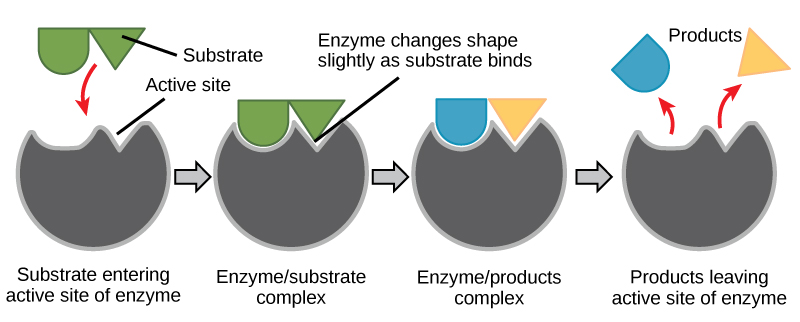
Ax and Ay are defined to be the components of A along the x- and y-axes. The three vectors A, Ax, and Ay form a right triangle:

Ax + Ay = A.
3.3

Note that this relationship between vector components and the resultant vector holds only for vector quantities (which include both magnitude and direction). The relationship does not apply for the magnitudes alone. For example, if Ax=3 m east, Ay=4 m north, and A=5 m north-east, then it is true that the vectors Ax + Ay = A. However, it is not true that the sum of the magnitudes of the vectors is also equal. That is,

3 m+4 m  ≠  5 m
3.4

Thus,

A x + A y ≠ A
3.5

If the vector A is known, then its magnitude A (its length) and its angle θ (its direction) are known. To find Ax and Ay, its x- and y-components, we use the following relationships for a right triangle.

A x = A cos θ
3.6

and

Ay=Asinθ.
3.7
]A dotted vector A sub x whose magnitude is equal to A cosine theta is drawn from the origin along the x axis. From the head of the vector A sub x another vector A sub y whose magnitude is equal to A sine theta is drawn in the upward direction. Their resultant vector A is drawn from the tail of the vector A sub x to the head of the vector A-y at an angle theta from the x axis. Therefore vector A is the sum of the vectors A sub x and A sub y.
Figure 3.25 — 3.3 Vector Addition and Subtraction: Analytical Methods

Figure 3.25 The magnitudes of the vector components A x A x and A y A y can be related to the resultant vector A A and the angle θ θ with trigonometric identities. Here we see that A x = A cos θ A x = A cos θ and A y = A sin θ A y = A sin θ .

Paul Peter Urone and Roger Hinrichs, College Physics 2E, OpenStax. · CC BY-NC-SA 4.0 · Original image ↗ · Access for free ↗
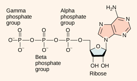
Suppose, for example, that A is the vector representing the total displacement of the person walking in a city considered in Kinematics in Two Dimensions: An Introduction and Vector Addition and Subtraction: Graphical Methods.

In the given figure a vector A of magnitude ten point three blocks is inclined at an angle twenty nine point one degrees to the positive x axis. The horizontal component A sub x of vector A is equal to A cosine theta which is equal to ten point three blocks multiplied to cosine twenty nine point one degrees which is equal to nine blocks east. Also the vertical component A sub y of vector A is equal to A sin theta is equal to ten point three blocks multiplied to sine twenty nine point one degrees,  which is equal to five point zero blocks north.
Figure 3.26 — 3.3 Vector Addition and Subtraction: Analytical Methods

Figure 3.26 We can use the relationships A x = A cos θ A x = A cos θ and A y = A sin θ A y = A sin θ to determine the magnitude of the horizontal and vertical component vectors in this example.

Paul Peter Urone and Roger Hinrichs, College Physics 2E, OpenStax. · CC BY-NC-SA 4.0 · Original image ↗ · Access for free ↗
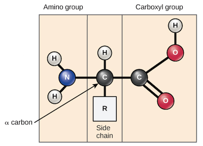
Then A=10.3 blocks and θ = 29.1º , so that

Ax=Acosθ=(10.3 blocks)(cos29.1º)=9.0 blocks
3.8
Ay=Asinθ=(10.3 blocks)(sin29.1º)=5.0 blocks.
3.9

Calculating a Resultant Vector

If the perpendicular components Ax and Ay of a vector A are known, then A can also be found analytically. To find the magnitude A and direction θ of a vector from its perpendicular components Ax and Ay, relative to the x-axis, we use the following relationships:

A= A x 2 + A y 2
3.10
θ = tan − 1 ( A y / A x ) .
3.11
Vector A is shown with its horizontal and vertical components A sub x and A sub y respectively. The magnitude of vector A is equal to the square root of A sub x squared plus A sub y squared. The angle theta of the vector A with the x axis is equal to inverse tangent of A sub y over A sub x
Figure 3.27 — 3.3 Vector Addition and Subtraction: Analytical Methods

Figure 3.27 The magnitude and direction of the resultant vector can be determined once the horizontal and vertical components A x A x and A y A y have been determined.

Paul Peter Urone and Roger Hinrichs, College Physics 2E, OpenStax. · CC BY-NC-SA 4.0 · Original image ↗ · Access for free ↗
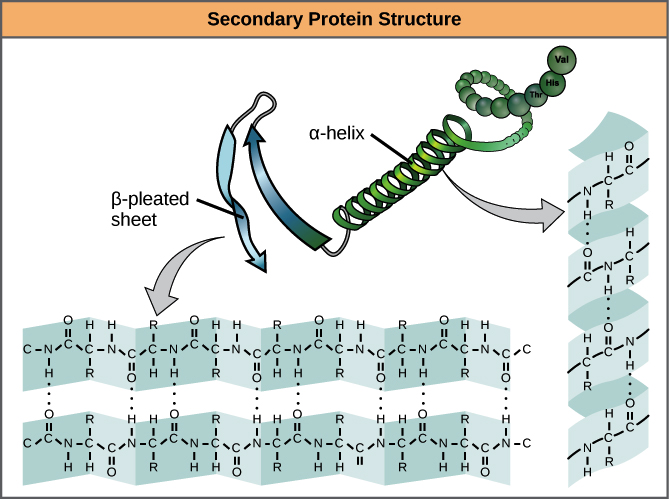
Note that the equation A = A x 2 + A y 2 is just the Pythagorean theorem relating the legs of a right triangle to the length of the hypotenuse. For example, if Ax and Ay are 9 and 5 blocks, respectively, then A=92+52=10.3 blocks, again consistent with the example of the person walking in a city. Finally, the direction is θ = tan –1 ( 5/9 ) =29.1º , as before.

Determining Vectors and Vector Components with Analytical Methods

Equations Ax=Acosθ and Ay=Asinθ are used to find the perpendicular components of a vector—that is, to go from A and θ to Ax and Ay. Equations A=Ax2+Ay2 and θ=tan–1(Ay/Ax) are used to find a vector from its perpendicular components—that is, to go from Ax and Ay to A and θ . Both processes are crucial to analytical methods of vector addition and subtraction.

Adding Vectors Using Analytical Methods

To see how to add vectors using perpendicular components, consider Figure 3.28, in which the vectors A and B are added to produce the resultant R.

Two vectors A and B are shown. The tail of vector B is at the head of vector A and the tail of the vector A is at origin. Both the vectors are in the first quadrant. The resultant R of these two vectors extending from the tail of vector A to the head of vector B is also shown.
Figure 3.28 — 3.3 Vector Addition and Subtraction: Analytical Methods

Figure 3.28 Vectors A A and B B are two legs of a walk, and R R is the resultant or total displacement. You can use analytical methods to determine the magnitude and direction of R R .

Paul Peter Urone and Roger Hinrichs, College Physics 2E, OpenStax. · CC BY-NC-SA 4.0 · Original image ↗ · Access for free ↗
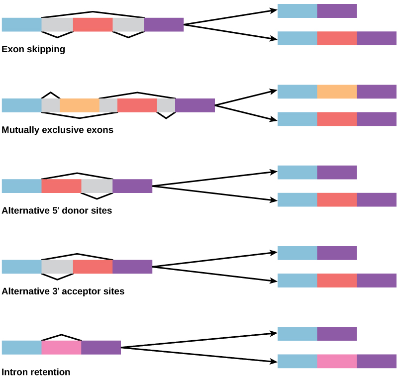
If A and B represent two legs of a walk (two displacements), then R is the total displacement. The person taking the walk ends up at the tip of R. There are many ways to arrive at the same point. In particular, the person could have walked first in the x-direction and then in the y-direction. Those paths are the x- and y-components of the resultant, Rx and Ry. If we know Rx and Ry, we can find R and θ using the equations A = A x 2 + Ay 2 and θ =tan –1 (Ay /Ax ). When you use the analytical method of vector addition, you can determine the components or the magnitude and direction of a vector.

Step 1. Identify the x- and y-axes that will be used in the problem. Then, find the components of each vector to be added along the chosen perpendicular axes. Use the equations Ax=Acosθ and Ay=Asinθ to find the components. In Figure 3.29, these components are Ax, Ay, Bx, and By. The angles that vectors A and B make with the x-axis are θA and θB, respectively.

Two vectors A and B are shown. The tail of the vector B is at the head of vector A and the tail of the vector A is at origin. Both the vectors are in the first quadrant. The resultant R of these two vectors extending from the tail of vector A to the head of vector B is also shown. The horizontal and vertical components of the vectors A and B are shown with the help of dotted lines. The vectors labeled as A sub x and A sub y are the components of vector A, and B sub x and B sub y as the components of vector B..
Figure 3.29 — 3.3 Vector Addition and Subtraction: Analytical Methods

Figure 3.29 To add vectors A A and B B , first determine the horizontal and vertical components of each vector. These are the dotted vectors A x A x , A y A y , B x B x and B y B y shown in the image.

Paul Peter Urone and Roger Hinrichs, College Physics 2E, OpenStax. · CC BY-NC-SA 4.0 · Original image ↗ · Access for free ↗
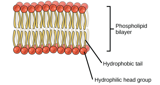
Step 2. Find the components of the resultant along each axis by adding the components of the individual vectors along that axis. That is, as shown in Figure 3.30,

R x = A x + B x
3.12

and

R y = A y + B y .
3.13
Two vectors A and B are shown. The tail of vector B is at the head of vector A and the tail of the vector A is at origin. Both the vectors are in the first quadrant. The resultant R of these two vectors extending from the tail of vector A to the head of vector B is also shown. The vectors A and B are resolved into the horizontal and vertical components shown as dotted lines parallel to x axis and y axis respectively. The horizontal components of vector A and vector B are labeled as A sub x and B sub x and the horizontal component of the resultant R is labeled at R sub x and is equal to A sub x plus B sub x. The vertical components of vector A and vector B are labeled as A sub y and B sub y and the vertical components of the resultant R is labeled as R sub y is equal to A sub y plus B sub y.
Figure 3.30 — 3.3 Vector Addition and Subtraction: Analytical Methods

Figure 3.30 The magnitude of the vectors A x A x and B x B x add to give the magnitude R x R x of the resultant vector in the horizontal direction. Similarly, the magnitudes of the vectors A y A y and B y B y add to give the magnitude R y R y of the resultant vector in the vertical direction.

Paul Peter Urone and Roger Hinrichs, College Physics 2E, OpenStax. · CC BY-NC-SA 4.0 · Original image ↗ · Access for free ↗
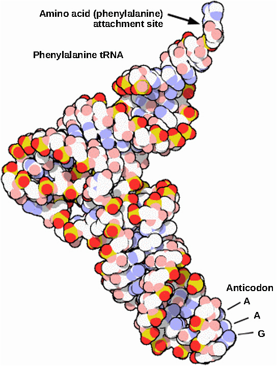
Components along the same axis, say the x-axis, are vectors along the same line and, thus, can be added to one another like ordinary numbers. The same is true for components along the y-axis. (For example, a 9-block eastward walk could be taken in two legs, the first 3 blocks east and the second 6 blocks east, for a total of 9, because they are along the same direction.) So resolving vectors into components along common axes makes it easier to add them. Now that the components of R are known, its magnitude and direction can be found.

Step 3. To get the magnitude R of the resultant, use the Pythagorean theorem:

R=Rx2+Ry2.
3.14

Step 4. To get the direction of the resultant relative to the x-axis:

θ=tan−1(Ry/Rx).
3.15

The following example illustrates this technique for adding vectors using perpendicular components.

Example 3.3

Adding Vectors Using Analytical Methods

Add the vector A to the vector B shown in Figure 3.31, using perpendicular components along the x- and y-axes. The x- and y-axes are along the east–west and north–south directions, respectively. Vector A represents the first leg of a walk in which a person walks 53.0 m in a direction 20.0º north of east. Vector B represents the second leg, a displacement of 34.0 m in a direction 63.0º north of east.

Two vectors A and B are shown. The tail of the vector A is at origin. Both the vectors are in the first quadrant. Vector A is of magnitude fifty three units and is inclined at an angle of twenty degrees to the horizontal. From the head of the vector A another vector B of magnitude 34 units is drawn and is inclined at angle sixty three degrees with the horizontal. The resultant of two vectors is drawn from the tail of the vector A to the head of the vector B.
Figure 3.31 — 3.3 Vector Addition and Subtraction: Analytical Methods

Figure 3.31 Vector A A has magnitude 53 . 0 m 53 . 0 m and direction 20 . 0 º 20 . 0 º north of the x -axis. Vector B B has magnitude 34 . 0 m 34 . 0 m and direction 63 . 0 º 63 . 0 º north of the x -axis. You can use analytical methods to determine the magnitude and direction of R R .

Paul Peter Urone and Roger Hinrichs, College Physics 2E, OpenStax. · CC BY-NC-SA 4.0 · Original image ↗ · Access for free ↗
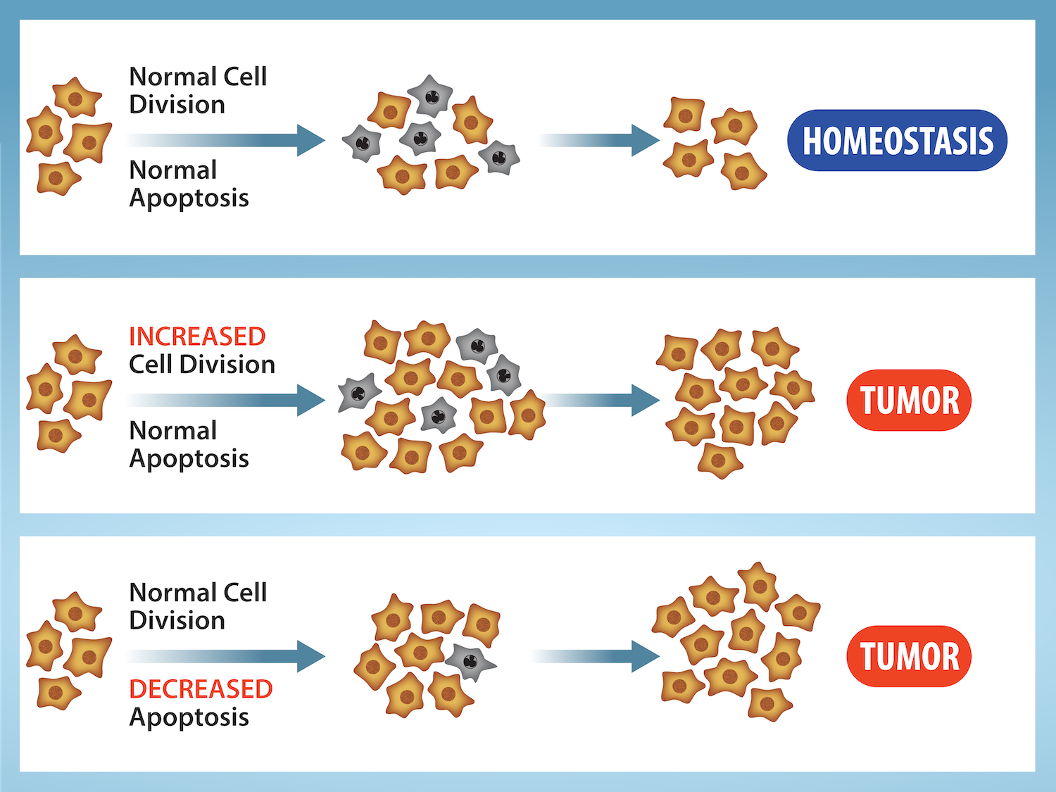
Strategy

The components of A and B along the x- and y-axes represent walking due east and due north to get to the same ending point. Once found, they are combined to produce the resultant.

Following the method outlined above, we first find the components of A and B along the x- and y-axes. Note that A=53.0 m, θA=20.0º, B=34.0 m, and θB=63.0º. We find the x-components by using Ax=Acosθ, which gives

A x = A cos θ A = ( 53. 0 m ) ( cos 20.0º ) = ( 53. 0 m ) ( 0 .940 ) = 49. 8 m
3.16

and

B x = B cos θ B = ( 34 . 0 m ) ( cos 63.0º ) = ( 34 . 0 m ) ( 0 . 454 ) = 15 . 4 m .
3.17

Similarly, the y-components are found using Ay=AsinθA:

A y = A sin θ A = ( 53 . 0 m ) ( sin 20.0º ) = ( 53 . 0 m ) ( 0 . 342 ) = 18 . 1 m
3.18

and

B y = B sin θ B = ( 34 . 0 m ) ( sin 63 . 0 º ) = ( 34 . 0 m ) ( 0 . 891 ) = 30 . 3 m .
3.19

The x- and y-components of the resultant are thus

R x = A x + B x = 49 . 8 m + 15 . 4 m = 65 . 2 m
3.20

and

Ry=Ay+By=18.1 m+30.3 m=48.4 m.
3.21

Now we can find the magnitude of the resultant by using the Pythagorean theorem:

R = R x 2 + R y 2 = ( 65 . 2 ) 2 + ( 48 . 4 ) 2 m
3.22

so that

R = 81.2 m.
3.23

Finally, we find the direction of the resultant:

θ=tan−1(Ry/Rx)=+tan−1(48.4/65.2).
3.24

Thus,

θ=tan−1(0.742)=36.6º.
3.25
The addition of two vectors A and B is shown. Vector A is of magnitude fifty three units and is inclined at an angle of twenty degrees to the horizontal. Vector B is of magnitude thirty four units and is inclined at angle sixty three degrees to the horizontal. The components of vector A are shown as dotted vectors A X is equal to forty nine point eight meter along x axis and A Y is equal to eighteen point one meter along Y axis. The components of vector B are also shown as dotted vectors B X is equal to fifteen point four meter and B Y is equal to thirty point three meter. The horizontal component of the resultant R X is equal to A X plus B X is equal to sixty five point two meter. The vertical component of the resultant R Y is equal to A Y plus B Y is equal to forty eight point four meter. The magnitude of the resultant of two vectors is eighty one point two meters. The direction of the resultant R is in thirty six point six degree from the vector A in anticlockwise direction.
Figure 3.32 — 3.3 Vector Addition and Subtraction: Analytical Methods

Figure 3.32 Using analytical methods, we see that the magnitude of R R is 81 . 2 m 81 . 2 m and its direction is 36 . 6º 36 . 6º north of east.

Paul Peter Urone and Roger Hinrichs, College Physics 2E, OpenStax. · CC BY-NC-SA 4.0 · Original image ↗ · Access for free ↗
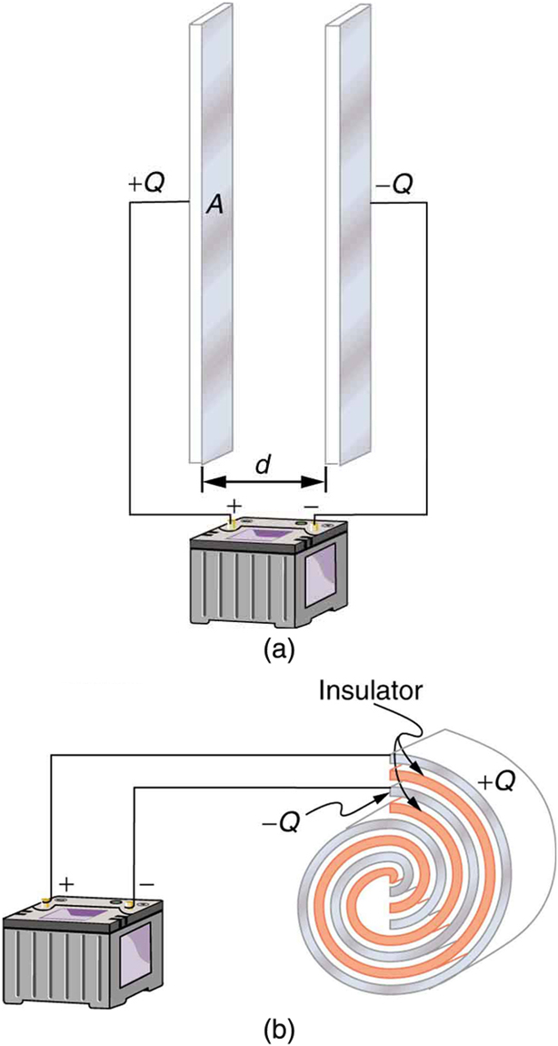
Discussion

This example illustrates the addition of vectors using perpendicular components. Vector subtraction using perpendicular components is very similar—it is just the addition of a negative vector.

Subtraction of vectors is accomplished by the addition of a negative vector. That is, A−B≡A+(–B). Thus, the method for the subtraction of vectors using perpendicular components is identical to that for addition. The components of –B are the negatives of the components of B. The x- and y-components of the resultant A−B = R are thus

R x = A x + (– B x )
3.26

and

R y = A y + (– B y )
3.27

and the rest of the method outlined above is identical to that for addition. (See Figure 3.33.)

Analyzing vectors using perpendicular components is very useful in many areas of physics, because perpendicular quantities are often independent of one another. The next module, Projectile Motion, is one of many in which using perpendicular components helps make the picture clear and simplifies the physics.

In this figure, the subtraction of two vectors A and B is shown. A red colored vector A is inclined at an angle theta A to the positive of x axis. From the head of vector A a blue vector negative B is drawn. Vector B is in west of south direction. The resultant of the vector A and vector negative B is shown as a black vector R from the tail of vector A to the head of vector negative B. The resultant R is inclined to x axis at an angle theta below the x axis. The components of the vectors are also shown along the coordinate axes as dotted lines of their respective colors.
Figure 3.33 — 3.3 Vector Addition and Subtraction: Analytical Methods

Figure 3.33 The subtraction of the two vectors shown in Figure 3.28 . The components of –B –B are the negatives of the components of B B . The method of subtraction is the same as that for addition.

Paul Peter Urone and Roger Hinrichs, College Physics 2E, OpenStax. · CC BY-NC-SA 4.0 · Original image ↗ · Access for free ↗
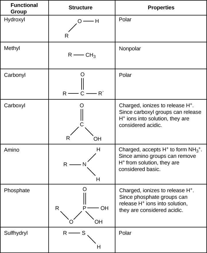
PhET Explorations

Vector Addition

Learn how to add vectors. Drag vectors onto a graph, change their length and angle, and sum them together. The magnitude, angle, and components of each vector can be displayed in several formats.

1.2 Physical Quantities and Units

OpenStax · 1.2 Physical Quantities and Units ↗
Instructional page including learning objectives, examples, figures, source tables and questions. Site navigation and embedded media players are omitted; source media links remain available.

Learning Objectives

By the end of this section, you will be able to:

  • Perform unit conversions both in the SI and English units.
  • Explain the most common prefixes in the SI units and be able to write them in scientific notation.
A view of Earth from the Moon.
Figure 1.15 — 1.2 Physical Quantities and Units

Figure 1.15 The distance from Earth to the Moon may seem immense, but it is just a tiny fraction of the distances from Earth to other celestial bodies. (credit: NASA)

Paul Peter Urone and Roger Hinrichs, College Physics 2E, OpenStax. (credit: NASA) · CC BY-NC-SA 4.0 · Original image ↗ · Access for free ↗
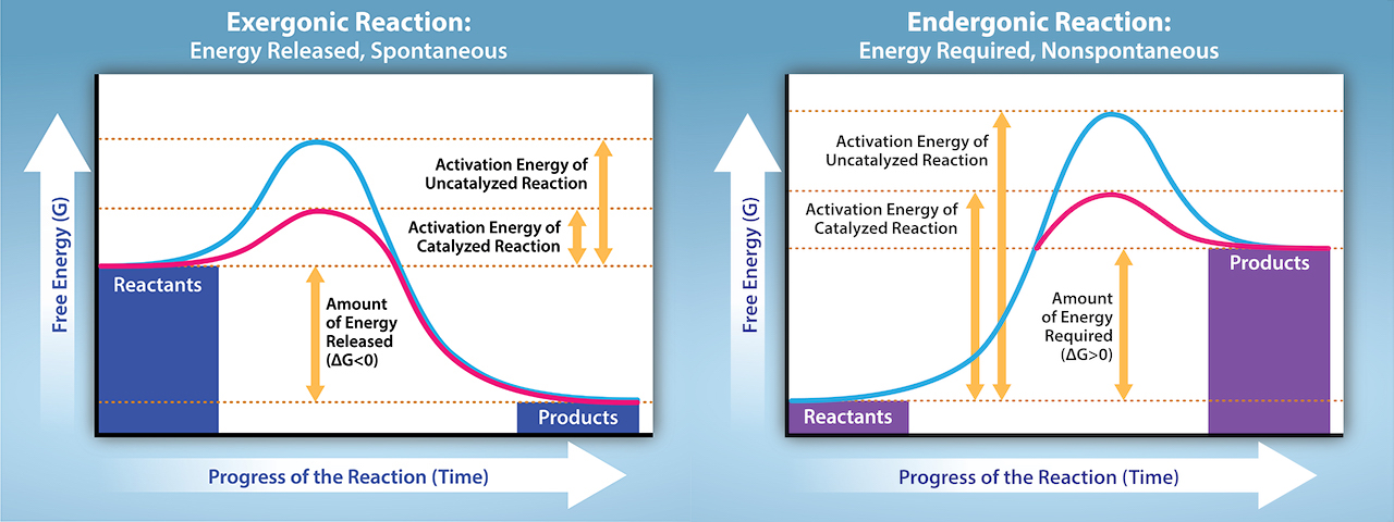
The range of objects and phenomena studied in physics is immense. From the incredibly short lifetime of a to the age of the Earth, from the tiny sizes of sub- particles to the vast distance to the edges of the known universe, from the force exerted by a jumping flea to the force between Earth and the Sun, there are enough factors of 10 to challenge the imagination of even the most experienced scientist. Giving numerical values for physical quantities and equations for physical principles allows us to understand nature much more deeply than does description alone. To comprehend these vast ranges, we must also have accepted units in which to express them. And we shall find that (even in the potentially mundane discussion of meters, kilograms, and seconds) a profound simplicity of nature appears—most physical quantities can be expressed as combinations of only four fundamental physical quantities: length, mass, time, and .

We define a physical quantity either by specifying how it is measured or by stating how it is calculated from other measurements. For example, we define distance and time by specifying methods for measuring them, whereas we define average speed by stating that it is calculated as distance traveled divided by time of travel.

Measurements of physical quantities are expressed in terms of units, which are standardized values. For example, the length of a race, which is a physical quantity, can be expressed in units of meters (for sprinters) or kilometers (for distance runners). Without standardized units, it would be extremely difficult for scientists to express and compare measured values in a meaningful way. (See Figure 1.16.)

A boy looking at a map and trying to guess distances with unit of length mentioned as cables between two points.
Figure 1.16 — 1.2 Physical Quantities and Units

Figure 1.16 Distances given in unknown units are maddeningly useless.

Paul Peter Urone and Roger Hinrichs, College Physics 2E, OpenStax. · CC BY-NC-SA 4.0 · Original image ↗ · Access for free ↗
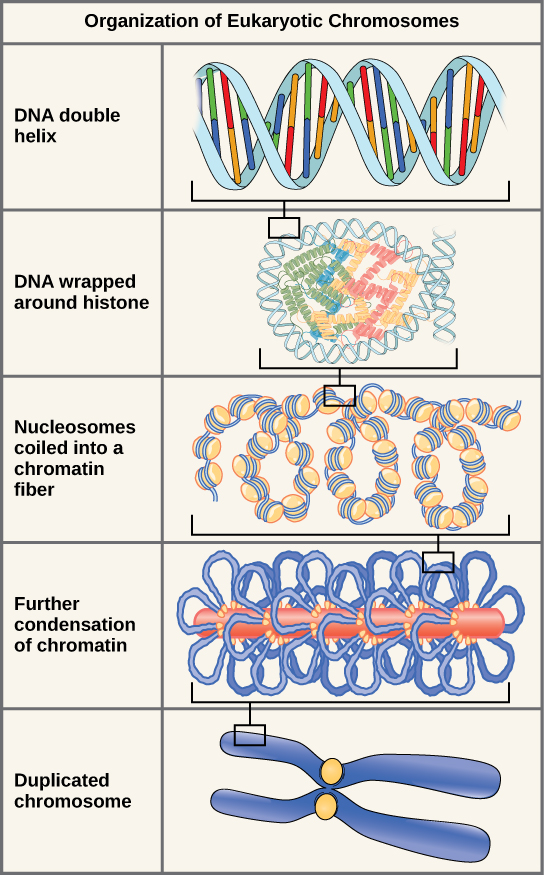
There are two major systems of units used in the world: SI units (also known as the metric system) and English units (also known as the customary or imperial system). English units were historically used in nations once ruled by the British Empire and are still widely used in the United States. Virtually every other country in the world now uses SI units as the standard; the metric system is also the standard system agreed upon by scientists and mathematicians. The acronym “SI” is derived from the French Système International.

SI Units: Fundamental and Derived Units

Table 1.1 gives the fundamental SI units that are used throughout this textbook. This text uses non-SI units in a few applications where they are in very common use, such as the measurement of blood pressure in millimeters of mercury (mm Hg). Whenever non-SI units are discussed, they will be tied to SI units through conversions.

Length Mass Time
meter (m) kilogram (kg) second (s) ampere (A)
Table 1.1 Fundamental SI Units

It is an intriguing that some physical quantities are more fundamental than others and that the most fundamental physical quantities can be defined only in terms of the procedure used to measure them. The units in which they are measured are thus called fundamental units. In this textbook, the fundamental physical quantities are taken to be length, mass, time, and . (Note that will not be introduced until much later in this text.) All other physical quantities, such as force and , can be expressed as algebraic combinations of length, mass, time, and current (for example, speed is length divided by time); these units are called derived units.

Units of Time, Length, and Mass: The Second, Meter, and Kilogram

The Second

The SI unit for time, the second (abbreviated s), has a long history. For many years it was defined as 1/86,400 of a mean solar day. More recently, a new standard was adopted to gain greater accuracy and to define the second in terms of a non-varying, or constant, physical phenomenon (because the solar day is getting longer due to very gradual slowing of the Earth’s rotation). Cesium can be made to vibrate in a very steady way, and these vibrations can be readily observed and counted. In 1967 the second was redefined as the time required for 9,192,631,770 of these vibrations. (See Figure 1.17.) Accuracy in the fundamental units is essential, because all measurements are ultimately expressed in terms of fundamental units and can be no more accurate than are the fundamental units themselves.

A top view of an atomic fountain is shown. It measures time using the vibration of the cesium atom.
Figure 1.17 — 1.2 Physical Quantities and Units

Figure 1.17 An atomic clock such as this one uses the vibrations of cesium atoms to keep time to a precision of better than a microsecond per year. The fundamental unit of time, the second, is based on such clocks. This image is looking down from the top of an atomic fountain nearly 30 feet tall! (credit: Steve Jurvetson/Flickr)

Paul Peter Urone and Roger Hinrichs, College Physics 2E, OpenStax. (credit: Steve Jurvetson/Flickr) · CC BY-NC-SA 4.0 · Original image ↗ · Access for free ↗

The Meter

The SI unit for length is the meter (abbreviated m); its definition has also changed over time to become more accurate and precise. The meter was first defined in 1791 as 1/10,000,000 of the distance from the equator to the North Pole. This measurement was improved in 1889 by redefining the meter to be the distance between two engraved lines on a platinum-iridium bar now kept near Paris. By 1960, it had become possible to define the meter even more accurately in terms of the of light, so it was again redefined as 1,650,763.73 of orange light emitted by krypton . In 1983, the meter was given its present definition (partly for greater accuracy) as the distance light travels in a vacuum in 1/299,792,458 of a second. (See Figure 1.18.) This change defines the speed of light to be exactly 299,792,458 meters per second. The length of the meter will change if the speed of light is someday measured with greater accuracy.

Beam of light from a flashlight is represented by an arrow pointing right, traveling the length of a meter stick.
Figure 1.18 — 1.2 Physical Quantities and Units

Figure 1.18 The meter is defined to be the distance light travels in 1/299,792,458 of a second in a vacuum. Distance traveled is speed multiplied by time.

Paul Peter Urone and Roger Hinrichs, College Physics 2E, OpenStax. · CC BY-NC-SA 4.0 · Original image ↗ · Access for free ↗
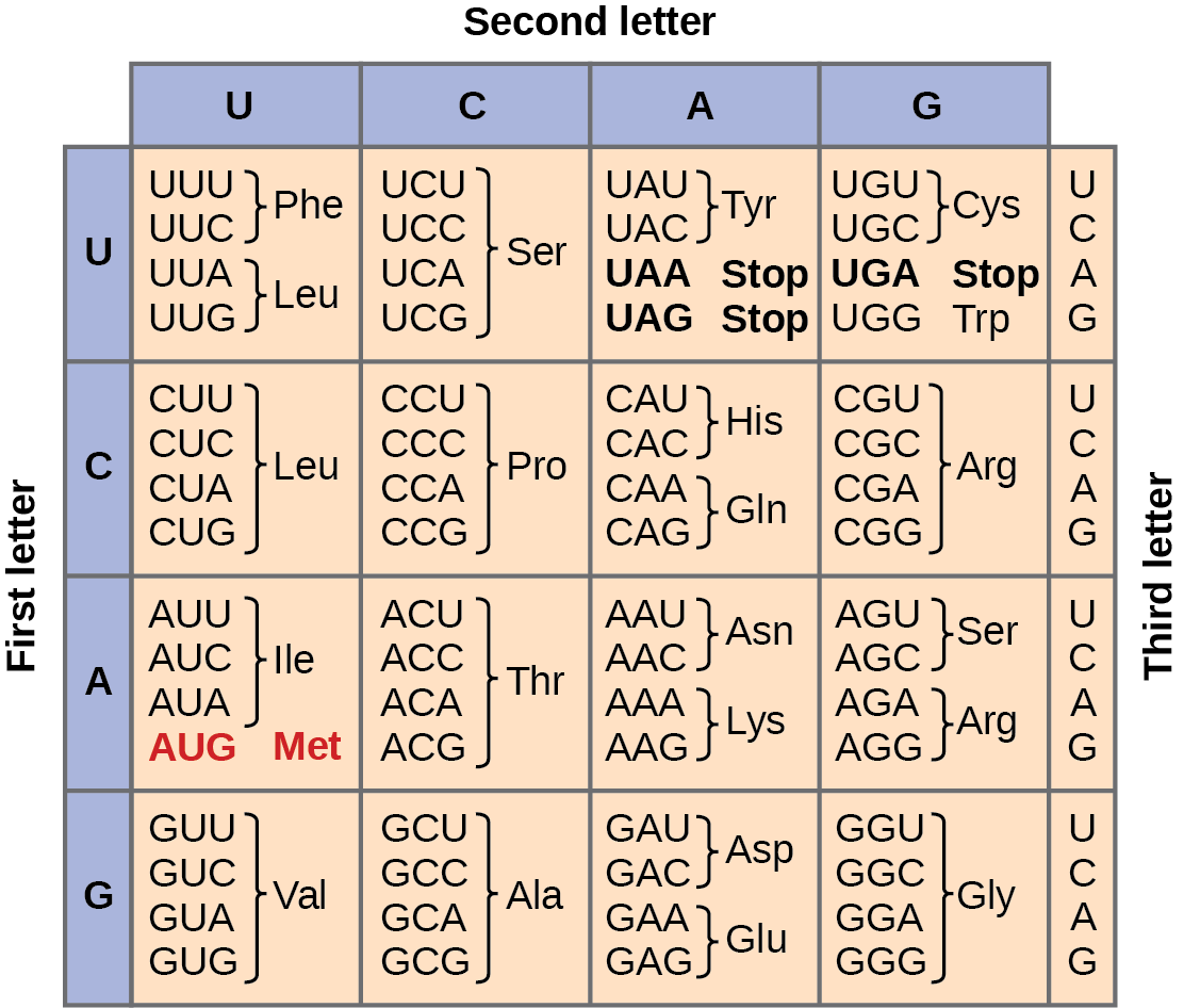
The Kilogram

The SI unit for mass is the kilogram (abbreviated kg); it was previously defined to be the mass of a platinum-iridium cylinder kept with the old meter standard at the International Bureau of Weights and Measures near Paris. Exact replicas of the previously defined kilogram are also kept at the United States’ National Institute of and Technology, or NIST, located in Gaithersburg, Maryland outside of Washington D.C., and at other locations around the world. The of all other masses could be ultimately traced to a comparison with the standard mass. Even though the platinum-iridium cylinder was resistant to corrosion, airborne contaminants were able to adhere to its surface, slightly changing its mass over time. In May 2019, the scientific community adopted a more stable definition of the kilogram. The kilogram is now defined in terms of the second, the meter, and Planck's constant, h (a quantum mechanical value that relates a 's energy to its frequency).

and its accompanying unit, the ampere, will be introduced in Electric Current, Resistance, and Ohm's Law when electricity and magnetism are covered. The initial modules in this textbook are concerned with mechanics, fluids, heat, and waves. In these subjects all pertinent physical quantities can be expressed in terms of the fundamental units of length, mass, and time.

Metric Prefixes

SI units are part of the metric system. The metric system is convenient for scientific and engineering calculations because the units are categorized by factors of 10. Table 1.2 gives metric prefixes and symbols used to denote various factors of 10.

Metric systems have the advantage that conversions of units involve only powers of 10. There are 100 centimeters in a meter, 1000 meters in a kilometer, and so on. In nonmetric systems, such as the system of U.S. customary units, the relationships are not as simple—there are 12 inches in a foot, 5280 feet in a mile, and so on. Another advantage of the metric system is that the same unit can be used over extremely large ranges of values simply by using an appropriate metric prefix. For example, distances in meters are suitable in construction, while distances in kilometers are appropriate for air travel, and the tiny measure of nanometers are convenient in optical design. With the metric system there is no need to invent new units for particular applications.

The term order of magnitude refers to the scale of a value expressed in the metric system. Each power of 10, and so forth are all different orders of magnitude. All quantities that can be expressed as a of a specific power of 10 are said to be of the same order of magnitude. For example, the number 800 can be written as 8×10², and the number 450 can be written as 4.5×10². Thus, the numbers 800 and 450 are of the same order of magnitude: 102. Order of magnitude can be thought of as a ballpark estimate for the scale of a value. The diameter of an is on the order of 10−10 m, while the diameter of the Sun is on the order of 109 m.

The Quest for Microscopic for Basic Units

The fundamental units described in this chapter are those that produce the greatest accuracy and precision in measurement. There is a sense among physicists that, because there is an underlying microscopic substructure to matter, it would be most satisfying to our of measurement on microscopic objects and fundamental physical phenomena such as the speed of light. A microscopic standard has been accomplished for the standard of time, which is based on the oscillations of the cesium .

The standard for length was once based on the of light (a small-scale length) emitted by a certain type of , but it has been supplanted by the more precise measurement of the speed of light. If it becomes possible to measure the mass of or a particular arrangement of such as a silicon sphere to greater precision than the kilogram standard, it may become possible to mass measurements on the small scale. There are also possibilities that electrical phenomena on the small scale may someday allow us to a unit of on the of and , but at present current and are related to large-scale currents and forces between wires.

Prefix Symbol Value Example (some are approximate)
exa E 10 18 exameter Em 10 18  m distance light travels in a century
peta P 10 15 petasecond Ps 10 15  s 30 million years
tera T 10 12 terawatt TW 10 12  W powerful laser output
giga G 10 9 gigahertz GHz 10 9  Hz a microwave frequency
mega M 10 6 megacurie MCi 10 6  Ci high radioactivity
kilo k 10 3 kilometer km 10 3  m about 6/10 mile
hecto h 10 2 hectoliter hL 10 2  L 26 gallons
deka da 10 1 dekagram 10 1  g teaspoon of butter
— — 100 (=1)
deci d 10 − 1 deciliter dL 10 − 1  L less than half a soda
centi c 10 − 2 10 − 2  m fingertip thickness
milli m 10 − 3 millimeter mm 10 − 3  m flea at its shoulders
micro µ 10 − 6 micrometer 10 − 6  m detail in microscope
nano n 10 − 9 nanogram ng 10 − 9  g small speck of dust
pico p 10 − 12 picofarad pF 10 − 12  F small in radio
femto f 10 − 15 femtometer fm 10 − 15  m size of a
atto a 10 − 18 attosecond as 10 − 18  s time light crosses an
Table 1.2 Metric Prefixes for Powers of 10 and their Symbols

Known Ranges of Length, Mass, and Time

The vastness of the universe and the breadth over which physics applies are illustrated by the wide range of examples of known lengths, masses, and times in Table 1.3. Examination of this table will give you some feeling for the range of possible topics and numerical values. (See Figure 1.19 and Figure 1.20.)

A magnified image of tiny phytoplankton swimming among the crystal of ice.[
Figure 1.19 — 1.2 Physical Quantities and Units

Figure 1.19 Tiny phytoplankton swims among crystals of ice in the Antarctic Sea. They range from a few micrometers to as much as 2 millimeters in length. (credit: Prof. Gordon T. Taylor, Stony Brook University; NOAA Corps Collections)

Paul Peter Urone and Roger Hinrichs, College Physics 2E, OpenStax. (credit: Prof. Gordon T. Taylor, Stony Brook University; NOAA Corps Collections) · CC BY-NC-SA 4.0 · Original image ↗ · Access for free ↗
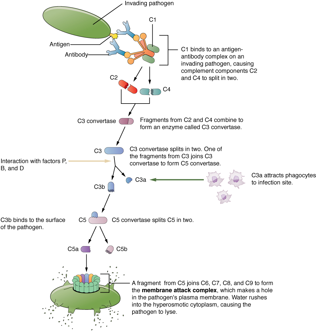
A view of Abell Galaxy with some bright stars and some hot gases.
Figure 1.20 — 1.2 Physical Quantities and Units

Figure 1.20 Galaxies collide 2.4 billion light years away from Earth. The tremendous range of observable phenomena in nature challenges the imagination. (credit: NASA/CXC/UVic./A. Mahdavi et al. Optical/lensing: CFHT/UVic./H. Hoekstra et al.)

Paul Peter Urone and Roger Hinrichs, College Physics 2E, OpenStax. (credit: NASA/CXC/UVic./A. Mahdavi et al. Optical/lensing: CFHT/UVic./H. Hoekstra et al.) · CC BY-NC-SA 4.0 · Original image ↗ · Access for free ↗
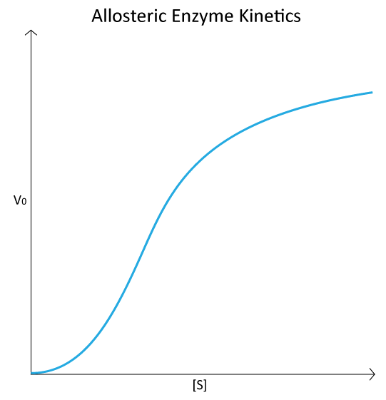
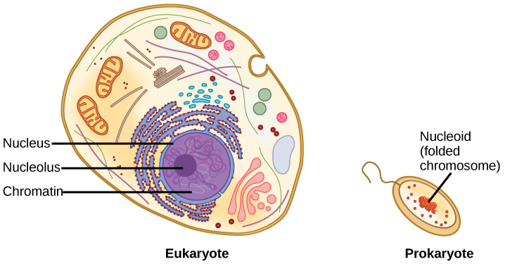
Unit Conversion and

It is often necessary to convert from one type of unit to another. For example, if you are reading a European cookbook, some quantities may be expressed in units of liters and you need to convert them to cups. Or, perhaps you are reading walking directions from one location to another and you are interested in how many miles you will be walking. In this case, you will need to convert units of feet to miles.

Let us consider a simple example of how to convert units. Let us say that we want to convert 80 meters (m) to kilometers (km).

The first thing to do is to list the units that you have and the units that you want to convert to. In this case, we have units in meters and we want to convert to kilometers.

Next, we need to determine a conversion factor relating meters to kilometers. A conversion factor is a ratio expressing how many of one unit are equal to another unit. For example, there are 12 inches in 1 foot, 100 centimeters in 1 meter, 60 seconds in 1 minute, and so on. In this case, we know that there are 1,000 meters in 1 kilometer.

Now we can set up our unit conversion. We will write the units that we have and then multiply them by the conversion factor so that the units cancel out, as shown:

80 m×1 km1000m=0.080 km.
1.1

Note that the unwanted m unit cancels, leaving only the desired km unit. You can use this method to convert between any types of unit.

Click Appendix C for a more complete list of conversion factors.

Lengths in meters Masses in kilograms (more precise values in parentheses) Times in seconds (more precise values in parentheses)
10 − 18 Present experimental limit to smallest observable detail 10 − 30 Mass of an 9.11×10⁻³¹ kg 10 − 23 Time for light to cross a
10 − 15 Diameter of a 10 − 27 Mass of a hydrogen 1.67×10⁻²⁷ kg 10 − 22 Mean life of an extremely unstable
10 − 14 Diameter of a uranium 10 − 15 Mass of a 10 − 15 Time for one oscillation of visible light
10 − 10 Diameter of a hydrogen 10 − 5 Mass of a mosquito 10 − 13 Time for one vibration of an in a solid
10 − 8 Thickness of in cells of living organisms 10 − 2 Mass of a hummingbird 10 − 8 Time for one oscillation of an FM radio wave
10 − 6 of visible light 1 Mass of a liter of water (about a quart) 10 − 3 Duration of a nerve impulse
10 − 3 Size of a grain of sand 10 2 Mass of a person 1 Time for one heartbeat
1 Height of a 4-year-old child 10 3 Mass of a car 10 5 One day 8.64×10⁴s
10 2 Length of a football field 10 8 Mass of a large ship 10 7 One year (y) 3.16×10⁷s
10 4 Greatest ocean depth 10 12 Mass of a large iceberg 10 9 About half the life expectancy of a human
10 7 Diameter of the Earth 10 15 Mass of the of a comet 10 11 Recorded history
10 11 Distance from the Earth to the Sun 10 23 Mass of the Moon 7.35×10²² kg 10 17 Age of the Earth
10 16 Distance traveled by light in 1 year (a light year) 10 25 Mass of the Earth 5.97×1024 kg 10 18 Age of the universe
10 21 Diameter of the Milky Way galaxy 10 30 Mass of the Sun 1.99×1030 kg
10 22 Distance from the Earth to the nearest large galaxy (Andromeda) 10 42 Mass of the Milky Way galaxy (current upper limit)
10 26 Distance from the Earth to the edges of the known universe 10 53 Mass of the known universe (current upper limit)
Table 1.3 Approximate Values of Length, Mass, and Time

Example 1.1

Unit Conversions: A Short Drive Home

Suppose that you drive the 10.0 km from your school to home in 20.0 min. Calculate your average speed (a) in kilometers per hour (km/h) and (b) in meters per second (m/s). (Note: Average speed is distance traveled divided by time of travel.)

Strategy

First we calculate the average speed using the given units. Then we can get the average speed into the desired units by picking the correct conversion factor and multiplying by it. The correct conversion factor is the one that cancels the unwanted unit and leaves the desired unit in its place.

for (a)

(1) Calculate average speed. Average speed is distance traveled divided by time of travel. (Take this definition as a given for now—average speed and other motion concepts will be covered in a later module.) In equation form,

average speed = distancetime.
1.2

(2) Substitute the given values for distance and time.

average speed = 10.0 km20.0 min=0.500 km min.
1.3

(3) Convert km/min to km/h: multiply by the conversion factor that will cancel minutes and leave hours. That conversion factor is 60 min/hr

Discussion for (a)

To check your answer, consider the following:

(1) Be sure that you have properly cancelled the units in the unit conversion. If you have written the unit conversion factor upside down, the units will not cancel properly in the equation. If you accidentally get the ratio upside down, then the units will not cancel; rather, they will give you the wrong units as follows:

 kmmin×1 hr60 min=160 km⋅hr min2,
1.4

which are obviously not the desired units of km/h.

(2) Check that the units of the final answer are the desired units. The problem asked us to solve for average speed in units of km/h and we have indeed obtained these units.

(3) Check the significant figures. Because each of the values given in the problem has three significant figures, the answer should also have three significant figures. The answer 30.0 km/ does indeed have three significant figures, so this is appropriate. Note that the significant figures in the conversion factor are not relevant because an hour is defined to be 60 minutes, so the precision of the conversion factor is perfect.

(4) Next, check whether the answer is reasonable. Let us consider some information from the problem—if you travel 10 km in a third of an hour (20 min), you would travel three times that far in an hour. The answer does seem reasonable.

for (b)

There are several ways to convert the average speed into meters per second.

(1) Start with the answer to (a) and convert km/h to m/s. Two conversion factors are needed—one to convert hours to seconds, and another to convert kilometers to meters.

(2) Multiplying by these yields

Average speed=30.0kmh×1h3,600 s×1,000m1 km,
1.5
Average speed=8.33ms.
1.6

Discussion for (b)

If we had started with 0.500 km/min, we would have needed different conversion factors, but the answer would have been the same: 8.33 m/s.

You may have noted that the answers in the worked example just covered were given to three digits. Why? When do you need to be concerned about the number of digits in something you calculate? Why not write down all the digits your calculator produces? The module Accuracy, Precision, and Significant Figures will help you answer these questions.

Nonstandard Units

While there are numerous types of units that we are all familiar with, there are others that are much more obscure. For example, a firkin is a unit of volume that was once used to measure beer. One firkin equals about 34 liters. To learn more about nonstandard units, use a dictionary or encyclopedia to research different “weights and measures.” Take note of any unusual units, such as a barleycorn, that are not listed in the text. Think about how the unit is defined and state its relationship to SI units.

Check Your Understanding

Some hummingbirds beat their wings more than 50 times per second. A scientist is measuring the time it takes for a hummingbird to beat its wings once. Which fundamental unit should the scientist use to describe the measurement? Which factor of 10 is the scientist likely to use to describe the motion precisely? Identify the metric prefix that corresponds to this factor of 10.

The scientist will measure the time between each movement using the fundamental unit of seconds. Because the wings beat so fast, the scientist will probably need to measure in milliseconds, or 10−3 seconds. (50 beats per second corresponds to 20 milliseconds per beat.)

Check Your Understanding

One cubic is equal to one milliliter. What does this tell you about the different units in the SI metric system?

The fundamental unit of length (meter) is probably used to create the derived unit of volume (liter). The measure of a milliliter is dependent on the measure of a .