Foundation 1 · 1C · Inheritance and genetic diversity

Population genetics and evolution

Sources ↗

Evolution changes heritable variation across generations; is a null model against which mechanisms and sampling can be tested.

calculations and assumptions

For two A and a, p+=1. Under random mating with a very large population and negligible , migration, and selection, expected frequencies are p², 2pq, and q². Count directly as p=(2NAA+NAa)/(2N). If a fully penetrant has frequency 0.01 under this model, =0.10, p=0.90, and carriers have frequency 0.18.

Do not equate an with a frequency. A departure from expected can reflect , selection, population mixture, or sampling; a single departure does not uniquely identify the mechanism. Sex-linked traits require accounting for different numbers of X copies.

Source: 19.1 Population Evolution · 19.2 Population Genetics · 19.3 Adaptive Evolution · 18.2 Formation of New Species

, , drift, and mating structure

creates new . Migration produces when migrants contribute genetically. is random sampling between generations, strongest in small populations; a reduces population size and a starts a population from few individuals, both potentially losing diversity. Drift can fix a harmful despite its cost.

increases and exposes variants, but by itself need not immediately change . can raise and reduce expression, though crossing strongly diverged populations can disrupt local . Nonrandom mating changes proportions; selection, , migration, and drift can change the underlying pool.

Source: 19.1 Population Evolution · 19.2 Population Genetics · 19.3 Adaptive Evolution · 18.2 Formation of New Species

, , and levels of selection

is relative contribution of viable, reproducing offspring in a specified environment, not strength or longevity alone. requires heritable variation associated with differential reproductive success. shifts a trait distribution, favors , and favors extremes. advantage or can maintain .

An improves reproductive success in its historical environment; specialization brings tradeoffs when conditions change. Selection can be analyzed at , organism, kin, or group levels, but a proposed group benefit must still explain differential persistence and reproduction. includes effects on relatives weighted by relatedness; it does not mean evolution consciously seeks species welfare.

Source: 19.1 Population Evolution · 19.2 Population Genetics · 19.3 Adaptive Evolution · 18.2 Formation of New Species

Isolation and divergence

Under the biological species concept, species are populations with effective reproductive isolation from others. prevent mating or fertilization, such as habitat, timing, behavior, and gametic incompatibility; reduce hybrid viability or fertility. Geographic separation can produce ; sympatric divergence can occur without a geographic barrier, including in plants.

Within-population is not itself . Reduced permits , drift, and selection to accumulate differences. Sequence differences can estimate divergence time when rates are available, but rates vary among and lineages. Molecular similarity reflects common ancestry, not a guaranteed constant evolutionary clock.

Source: 19.1 Population Evolution · 19.2 Population Genetics · 19.3 Adaptive Evolution · 18.2 Formation of New Species

Separate evidence from sampling noise

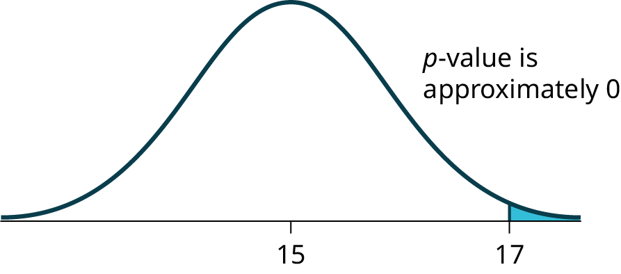
A finite offspring sample rarely matches an exact Mendelian ratio. Compare observed and expected counts with =(O−E)²/E when categories and expected counts support the approximation; degrees of freedom reflect independent categories minus constraints and estimated parameters. A small indicates that data are unusual under the specified null, not that a particular alternative is proven.

Larger samples narrow sampling uncertainty but do not remove biased recruitment or . Use independent observations and . In population association studies, ancestry can confound – relationships; , family designs, and mechanistic evidence help distinguish association from causal effects.

Source: 19.1 Population Evolution · 19.2 Population Genetics · 19.3 Adaptive Evolution · 18.2 Formation of New Species

Practice: apply the mechanism

Question. In a randomly mating population at , a affects 1 in 2,500 people. Estimate frequency. Separately, an Aa × Aa cross produces 90 and 30 offspring; what is for the 3:1 null?

Show reasoning

q²=1/2500=0.0004, so =0.02 and p=0.98. frequency=2pq=0.0392, about 3.92% or 1 in 25.5. For 120 offspring, the 3:1 null predicts 90 and 30 exactly, so =0. This agrees with the model in this sample but does not prove , equal viability, or any proposed molecular mechanism.

Source: 19.1 Population Evolution · 19.2 Population Genetics · 19.3 Adaptive Evolution · 18.2 Formation of New Species

19.1 Population Evolution — figures and tables
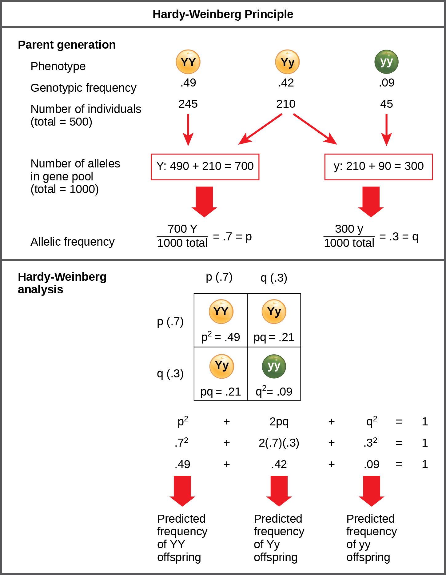
The Hardy-Weinberg principle is used to predict the genotypic distribution of offspring in a given population. In the example given, pea plants have two different alleles for pea color. The dominant capital Y allele results in yellow pea color, and the recessive small y allele results in green pea color. The distribution of individuals in a population of 500 is given. Of the 500 individuals, 245 are homozygous dominant (capital Y capital Y) and produce yellow peas. 210 are heterozygous (capital Y small y) and also produce yellow peas. 45 are homozygous recessive (small y small y) and produce green peas. The frequencies of homozygous dominant, heterozygous, and homozygous recessive individuals are 0.49, 0.42, and 0.09, respectively. Each of the 500 individuals provides two alleles to the gene pool, or 1000 total. The 245 homozygous dominant individuals provide two capital Y alleles to the gene pool, or 490 total. The 210 heterozygous individuals provide 210 capital Y and 210 small y alleles to the gene pool. The 45 homozygous recessive individuals provide two small y alleles to the gene pool, or 90 total. The number of capital Y alleles is 490 from homozygous dominant individuals plus 210 from homozygous recessive individuals, or 700 total. The number of small y alleles is 210 from heterozygous individuals plus 90 from homozygous recessive individuals, or 300 total. The allelic frequency is calculated by dividing the number of each allele by the total number of alleles in the gene pool. For the capital Y allele, the allelic frequency is 700 divided by 1000, or 0.7; this allelic frequency is called p. For the small y allele the allelic frequency is 300 divided by 1000, or 0.3; the allelic frequency is called q. Hardy-Weinberg analysis is used to determine the genotypic frequency in the offspring. The Hardy-Wienberg equation is p-squared plus 2pq plus q-squared equals 1. For the population given, the frequency is 0.7-squared plus 2 times .7 times .3 plus .3-squared equals one. The value for p-squared, 0.49, is the predicted frequency of homozygous dominant (capital Y capital Y) individuals. The value for 2pq, 0.42, is the predicted frequency of heterozygous (capital Y small y) individuals. The value for q-squared, .09, is the predicted frequency of homozygous recessive individuals. Note that the predicted frequency of genotypes in the offspring is the same as the frequency of genotypes in the parent population. If all the genotypic frequencies, .49 plus .42 plus .09, are added together, the result is one.
Figure 19.2 — 19.1 Population Evolution

Figure 19.2 When populations are in the Hardy-Weinberg equilibrium, the allelic frequency is stable from generation to generation and we can determine the allele distribution from the Hardy-Weinberg equation. If the allelic frequency measured in the field differs from the predicted value, scientists can make inferences about what evolutionary forces are at play.

Mary Ann Clark, Matthew Douglas, and Jung Choi, Biology 2E, OpenStax. · CC BY-NC-SA 4.0 · Original image ↗ · Access for free ↗

Source: 19.1 Population Evolution

19.2 Population Genetics — figures and tables
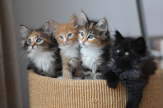
This photo shows four kittens in a basket: two are gray, black, orange, and white, the third cat is orange and white, and the fourth cat is black.
Figure 19.3 — 19.2 Population Genetics

Figure 19.3 The distribution of phenotypes in this litter of kittens illustrates population variation. (credit: Pieter Lanser)

Mary Ann Clark, Matthew Douglas, and Jung Choi, Biology 2E, OpenStax. (credit: Pieter Lanser) · CC BY-NC-SA 4.0 · Original image ↗ · Access for free ↗
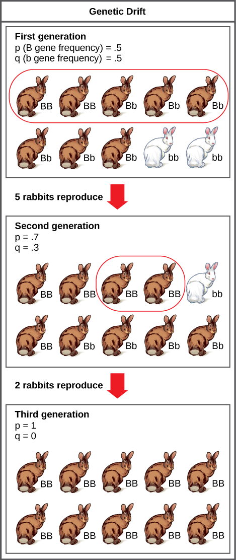
A population has 10 rabbits. 2 of these rabbits are homozygous dominant for the B allele and have brown coat color. 6 are heterozygous and also have brown coat color. Two are homozygous recessive and have white coat color. The frequency of the capital B allele, p, is .5 and the frequency of the small b allele, q, is also .5. Only 5 of the rabbits, including 2 homozygous dominant and 3 heterozygous individuals, produce offspring. 5 of the resulting offspring are homozygous dominant, 4 are heterozygous, and 1 is homozygous recessive. The frequency of alleles in the second generation is p=.7 and q=.3. Only 2 rabbits in the second generation produce offspring, and both of these are homozygous dominant. As a result, the recessive small b allele is lost in the third generation, and all of the rabbits are heterozygous dominant with brown coat color.
Figure 19.4 — 19.2 Population Genetics

Figure 19.4 Genetic drift in a population can lead to eliminating an allele from a population by chance. In this example, rabbits with the brown coat color allele ( B ) are dominant over rabbits with the white coat color allele ( b ). In the first generation, the two alleles occur with equal frequency in the population, resulting in p and q values of .5. Only half of the individuals reproduce, resulting in a second generation with p and q values of .7 and .3, respectively. Only two individuals in the second generation reproduce, and by chance these individuals are homozygous dominant for brown coat color. As a result, in the third generation the recessive b allele is lost.

Mary Ann Clark, Matthew Douglas, and Jung Choi, Biology 2E, OpenStax. · CC BY-NC-SA 4.0 · Original image ↗ · Access for free ↗
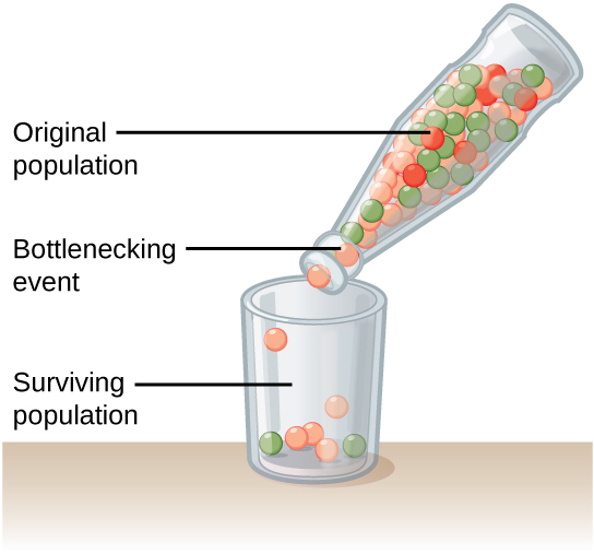
This illustration shows a narrow-neck bottle filled with red, orange, and green marbles. The bottle is tipped so the marbles pour into a glass. Because of the bottleneck, only seven marbles escape, and these are all orange and green. The marbles in the bottle represent the original population, and the marbles in the glass represent the surviving population. Because of the bottleneck effect, the surviving population is less diverse than the original population.
Figure 19.5 — 19.2 Population Genetics

Figure 19.5 A chance event or catastrophe can reduce the genetic variability within a population.

Mary Ann Clark, Matthew Douglas, and Jung Choi, Biology 2E, OpenStax. · CC BY-NC-SA 4.0 · Original image ↗ · Access for free ↗
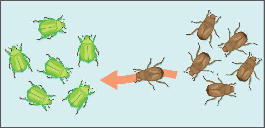
This illustration shows an individual from a population of brown insects traveling toward a population of green insects.
Figure 19.6 — 19.2 Population Genetics

Figure 19.6 Gene flow can occur when an individual travels from one geographic location to another.

Mary Ann Clark, Matthew Douglas, and Jung Choi, Biology 2E, OpenStax. · CC BY-NC-SA 4.0 · Original image ↗ · Access for free ↗
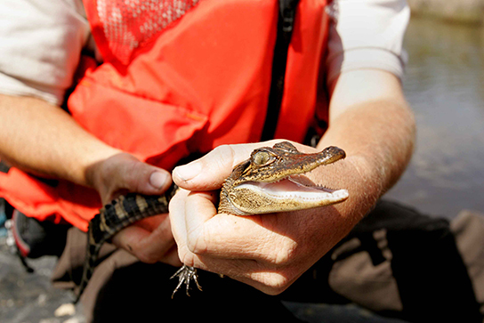
This photo shows a person holding a baby alligator.
Figure 19.7 — 19.2 Population Genetics

Figure 19.7 The temperature at which the eggs are incubated determine the American alligator's ( Alligator mississippiensis ) sex. Eggs incubated at 30°C produce females, and eggs incubated at 33°C produce males. (credit: Steve Hillebrand, USFWS)

Mary Ann Clark, Matthew Douglas, and Jung Choi, Biology 2E, OpenStax. (credit: Steve Hillebrand, USFWS) · CC BY-NC-SA 4.0 · Original image ↗ · Access for free ↗

Source: 19.2 Population Genetics

19.3 Adaptive Evolution — figures and tables
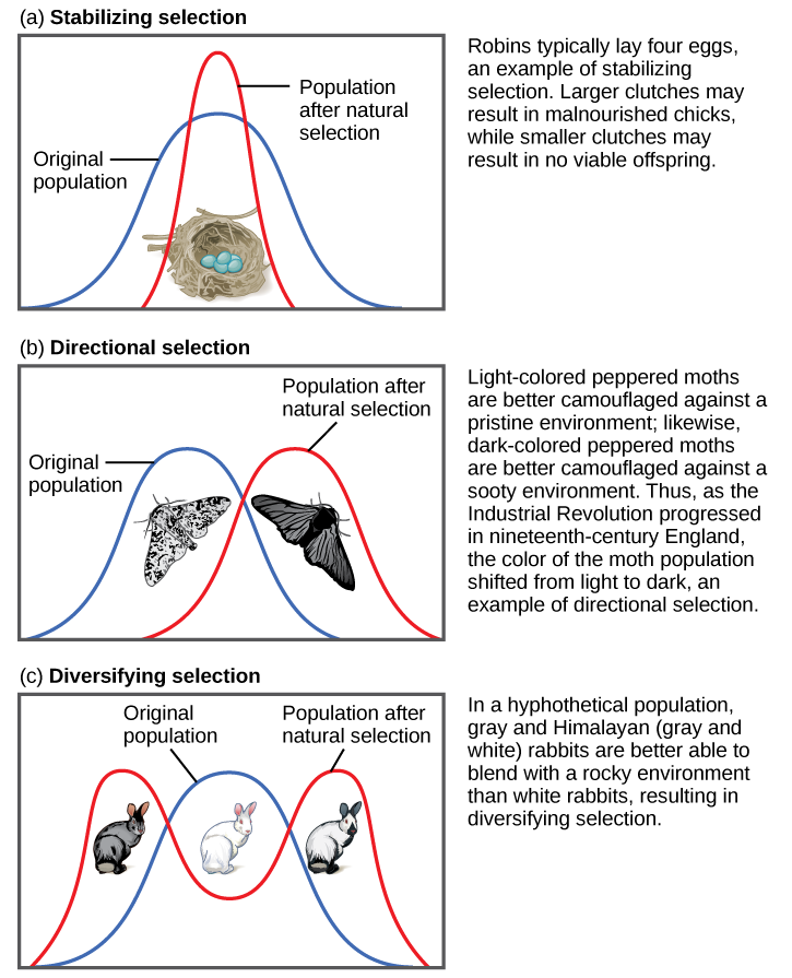
Part (a) shows a robin clutch size as an example of stabilizing selection. Robins typically lay four eggs. Larger clutches may result in malnourished chicks, while smaller clutches may result in no viable offspring. A wide bell curve indicates that, in the original population, there was a lot of variability in clutch size. Overlaying this wide bell curve is a narrow one that represents the clutch size after natural selection, which is much less variable. Part (b) shows moth color as an example of directional selection. Light-colored pepper moths are better camouflaged against a pristine environment, while dark-colored peppered moths are better camouflaged against a sooty environment. Thus, as the Industrial Revolution progressed in nineteenth-century England, the color of the moth population shifted from light to dark, an example of directional selection. A bell curve representing the original population and one representing the population after natural selection only slightly overlap. Part (c) shows rabbit coat color as an example of diversifying selection. In this hypothetical example, gray and Himalayan (gray and white) rabbits are better able to blend into their rocky environment than white ones. The original population is represented by a bell curve in which white is the most common coat color, while gray and Himalayan colors, on the right and left flank of the curve, are less common. After natural selection, the bell curve splits into two peaks, indicating gray and Himalayan coat color have become more common than the intermediate white coat color.
Figure 19.8 — 19.3 Adaptive Evolution

Figure 19.8 Different types of natural selection can impact the distribution of phenotypes within a population. In (a) stabilizing selection, an average phenotype is favored. In (b) directional selection, a change in the environment shifts the spectrum of observed phenotypes. In (c) diversifying selection, two or more extreme phenotypes are selected for, while the average phenotype is selected against.

Mary Ann Clark, Matthew Douglas, and Jung Choi, Biology 2E, OpenStax. · CC BY-NC-SA 4.0 · Original image ↗ · Access for free ↗
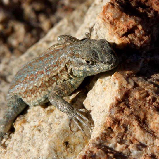
Photo shows a mottled green and brown lizard sitting on a rock.
Figure 19.9 — 19.3 Adaptive Evolution

Figure 19.9 A yellow-throated side-blotched lizard is smaller than either the blue-throated or orange-throated males and appears a bit like the females of the species, allowing it to sneak copulations. (credit: “tinyfroglet”/Flickr)

Mary Ann Clark, Matthew Douglas, and Jung Choi, Biology 2E, OpenStax. (credit: “tinyfroglet”/Flickr) · CC BY-NC-SA 4.0 · Original image ↗ · Access for free ↗
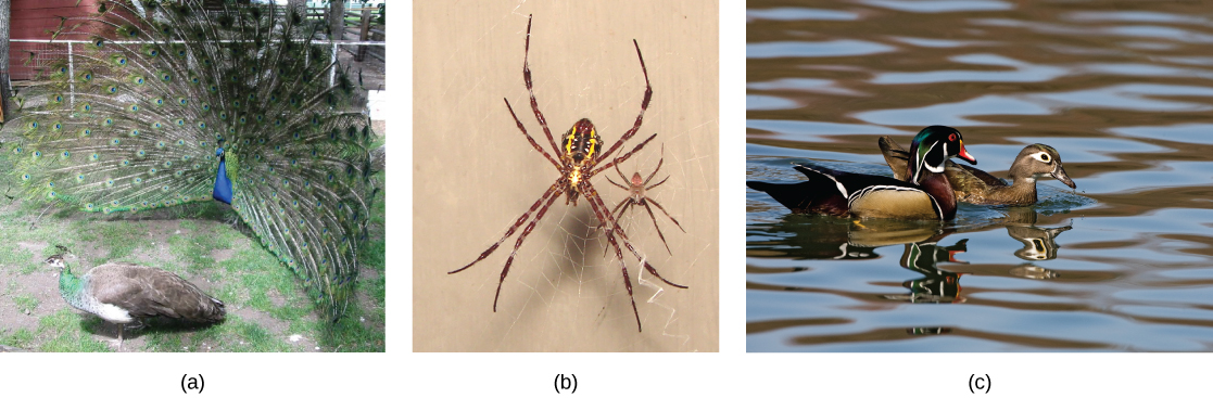
The photo on the left shows a peacock with a bright blue body and flared tail feathers standing next to a brown, drab peahen. The middle photo shows a large female spider sitting on a web next to its much smaller male counterpart. The photo on the right shows a brightly colored male wood duck swimming next to a drab brown female.
Figure 19.10 — 19.3 Adaptive Evolution

Figure 19.10 Sexual dimorphism in (a) peacocks and peahens, (b) Argiope appensa spiders (the female spider is the large one), and in (c) wood ducks. (credit “spiders”: modification of work by “Sanba38”/Wikimedia Commons; credit “duck”: modification of work by Kevin Cole)

Mary Ann Clark, Matthew Douglas, and Jung Choi, Biology 2E, OpenStax. (credit “spiders”: modification of work by “Sanba38”/Wikimedia Commons; credit “duck”: modification of work by Kevin Cole) · CC BY-NC-SA 4.0 · Original image ↗ · Access for free ↗

Source: 19.3 Adaptive Evolution

18.2 Formation of New Species — figures and tables
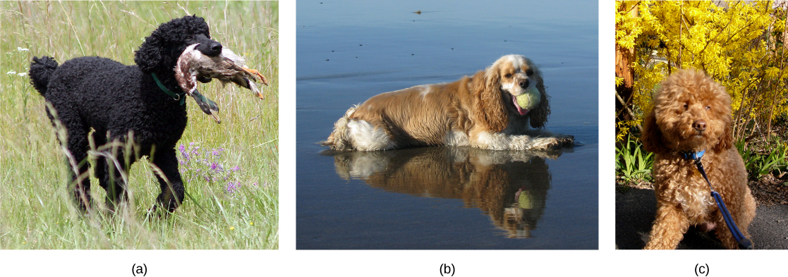
Photo a shows a poodle with curly short fur. Photo b shows a cocker spaniel with long, wavy fur that has light brown parts and cream-colored markings on the face, forepaws, belly, hind legs, and tail. The poodle has longer legs than the cocker spaniel. The cockapoo in photo c has curly hair, like the poodle, and short legs, like the cocker spaniel.
Figure 18.9 — 18.2 Formation of New Species

Figure 18.9 The (a) poodle and (b) cocker spaniel can reproduce to produce a breed known as (c) the cockapoo. (credit a: modification of work by Sally Eller, Tom Reese; credit b: modification of work by Jeremy McWilliams; credit c: modification of work by Kathleen Conklin)

Mary Ann Clark, Matthew Douglas, and Jung Choi, Biology 2E, OpenStax. (credit a: modification of work by Sally Eller, Tom Reese; credit b: modification of work by Jeremy McWilliams; credit c: modification of work by Kathleen Conklin) · CC BY-NC-SA 4.0 · Original image ↗ · Access for free ↗
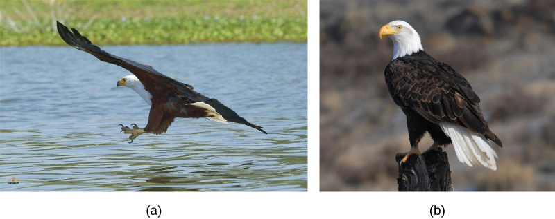
Photo a shows a picture of the African fish eagle in flight, and photo b shows the bald eagle perched on a post.  Both birds have dark brown feathers on their bodies and wings, and white feathered heads.
Figure 18.10 — 18.2 Formation of New Species

Figure 18.10 The (a) African fish eagle is similar in appearance to the (b) bald eagle, but the two birds are members of different species. (credit a: modification of work by Nigel Wedge; credit b: modification of work by U.S. Fish and Wildlife Service)

Mary Ann Clark, Matthew Douglas, and Jung Choi, Biology 2E, OpenStax. (credit a: modification of work by Nigel Wedge; credit b: modification of work by U.S. Fish and Wildlife Service) · CC BY-NC-SA 4.0 · Original image ↗ · Access for free ↗
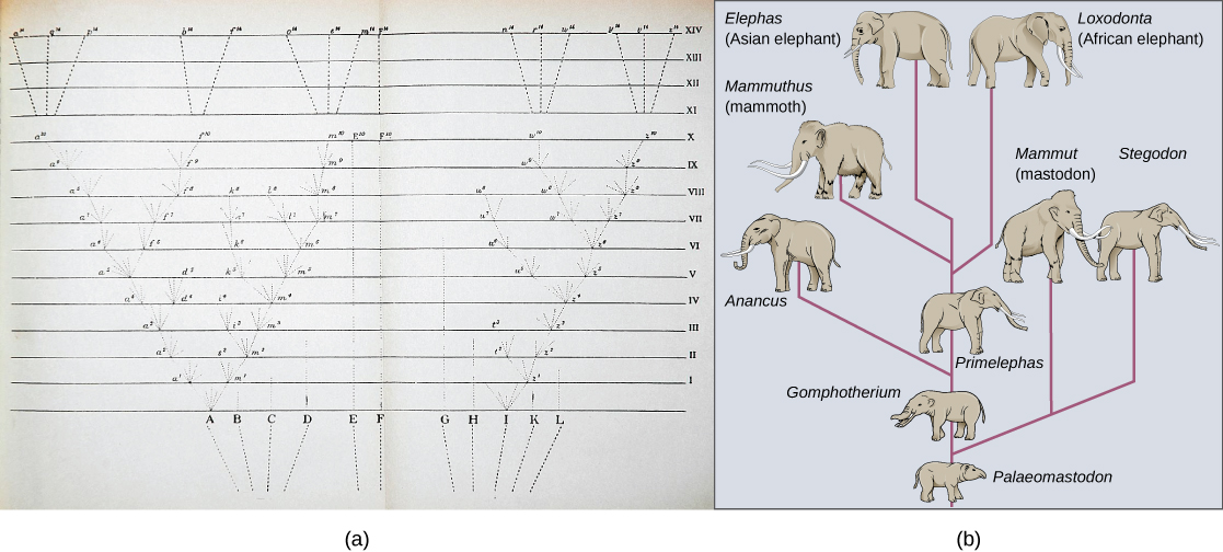
Image (a) shows a sketch of lines branching into a tree shape. At the bottom are 11 vertical lines labeled A through L. These then are branched out as they move up across the page through fourteen rows labeled with Roman numerals. Some branches make a straight line from the bottom row to the top row, others keep branching out further at each row, and some are straight partway through the rows until they connect to an existing branch or form no connection and instead stop. The top four rows contain lines branching out from 6 locations on row 11 to 15 individual final designations on row 14. Illustration B shows the evolution of modern African and Asian elephants from a common ancestor, the Palaeomastodon. The Palaeomastodon was similar to modern elephants; however, it was smaller and had a long nose instead of a trunk. Side branches of the elephant evolutionary tree gave rise to mastodons and mammoths. The mammoth is more closely related to modern elephants than the mastodon.
Figure 18.11 — 18.2 Formation of New Species

Figure 18.11 The only illustration in Darwin's On the Origin of Species is (a) a diagram showing speciation events leading to biological diversity. The diagram shows similarities to phylogenetic charts that today illustrate the relationships of species. (b) Modern elephants evolved from the Palaeomastodon , a species that lived in Egypt 35–50 million years ago.

Mary Ann Clark, Matthew Douglas, and Jung Choi, Biology 2E, OpenStax. · CC BY-NC-SA 4.0 · Original image ↗ · Access for free ↗
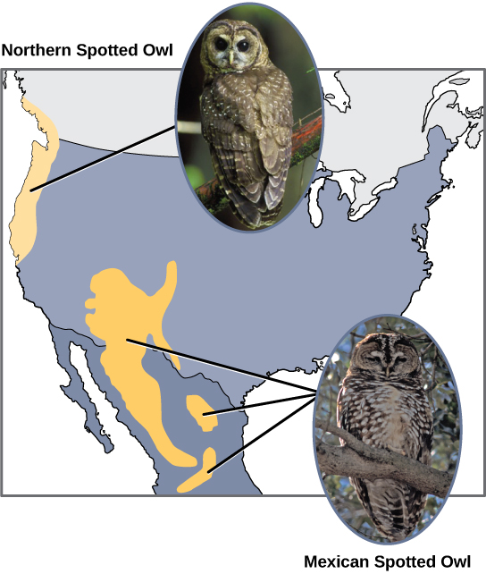
The northern spotted owl lives in the Pacific Northwest, and the Mexican spotted owl lives in Mexico and the southwestern portion of the United States. The two owls are similar in appearance but with slightly different coloration.
Figure 18.12 — 18.2 Formation of New Species

Figure 18.12 The northern spotted owl and the Mexican spotted owl inhabit geographically separate locations with different climates and ecosystems. The owl is an example of allopatric speciation. (credit "northern spotted owl": modification of work by John and Karen Hollingsworth; credit "Mexican spotted owl": modification of work by Bill Radke)

Mary Ann Clark, Matthew Douglas, and Jung Choi, Biology 2E, OpenStax. (credit "northern spotted owl": modification of work by John and Karen Hollingsworth; credit "Mexican spotted owl": modification of work by Bill Radke) · CC BY-NC-SA 4.0 · Original image ↗ · Access for free ↗
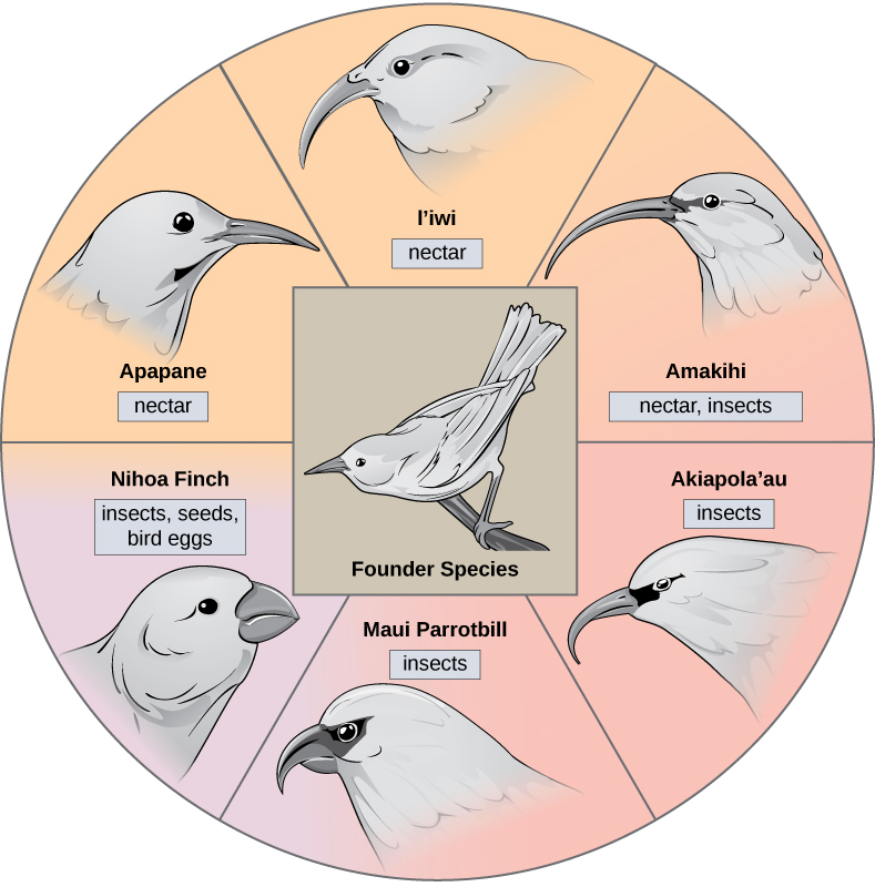
The illustration shows a wheel with the founder species at the hub. The spokes of the wheel are six modern honeycreeper bird species that evolved from the founder bird species. Five of these birds eat insects and or nectar and have long, thick beaks; these are the ‘Apapane, ‘Iwi, ‘Amakihi, ‘Akiapola'au and Maui Parrotbill. The Nihoa Finch has a short, fat beak and eats insects, seeds, and bird eggs.
Figure 18.13 — 18.2 Formation of New Species

Figure 18.13 The honeycreeper birds illustrate adaptive radiation. From one original species of bird, multiple others evolved, each with its own distinctive characteristics.

Mary Ann Clark, Matthew Douglas, and Jung Choi, Biology 2E, OpenStax. · CC BY-NC-SA 4.0 · Original image ↗ · Access for free ↗
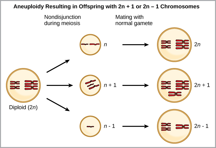
Aneuploidy results when chromosomes fail to separate correctly during meiosis. As a result, one gamete has one too many chromosomes, shown as n plus 1, and the other has one too few, shown as n minus 1. When the n + 1 gamete fuses with a normal gamete, the resulting zygote has 2 n + 1 chromosomes. When the n minus 1 gamete fuses with a normal gamete, the resulting zygote has 2 n minus 1 chromosomes.
Figure 18.14 — 18.2 Formation of New Species

Figure 18.14 Aneuploidy results when the gametes have too many or too few chromosomes due to nondisjunction during meiosis. In this example, the resulting offspring will have 2 n +1 or 2 n -1 chromosomes.

Mary Ann Clark, Matthew Douglas, and Jung Choi, Biology 2E, OpenStax. · CC BY-NC-SA 4.0 · Original image ↗ · Access for free ↗
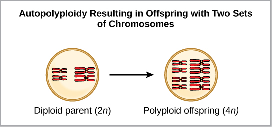
Autopolyploidy results in offspring with two sets of chromosomes. In the example shown, a diploid parent, 2 n produces polyploid offspring 4 n.
Figure 18.15 — 18.2 Formation of New Species

Figure 18.15 Autopolyploidy results when mitosis is not followed by cytokinesis.

Mary Ann Clark, Matthew Douglas, and Jung Choi, Biology 2E, OpenStax. · CC BY-NC-SA 4.0 · Original image ↗ · Access for free ↗
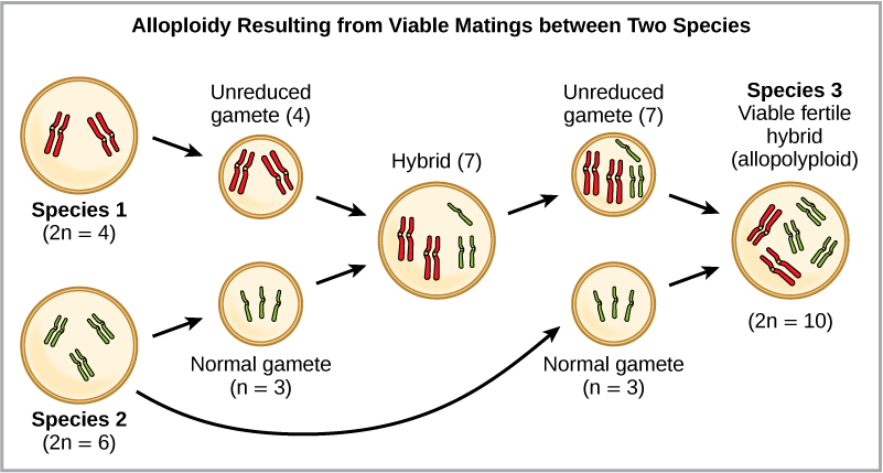
Alloploidy results from viable matings between two species with different numbers of chromosomes. In the example shown, species one has two pairs of chromosomes, and species two has three pairs of chromosomes. When an unreduced gamete from species one (with two pairs of chromosomes) fuses with a normal gamete from species two (with three unpaired chromosomes), a hybrid zygote with seven chromosomes results. An offspring from this mating produces an unreduced gamete with seven chromosomes. If this unreduced gamete fuses with a normal gamete from species one, with three chromosomes, the resulting offspring will have ten viable chromosomes (five pairs of chromosomes).
Figure 18.16 — 18.2 Formation of New Species

Figure 18.16 Alloploidy results when two species mate to produce viable offspring. In this example, a normal gamete from one species fuses with a polyploidy gamete from another. Two matings are necessary to produce viable offspring.

Mary Ann Clark, Matthew Douglas, and Jung Choi, Biology 2E, OpenStax. · CC BY-NC-SA 4.0 · Original image ↗ · Access for free ↗
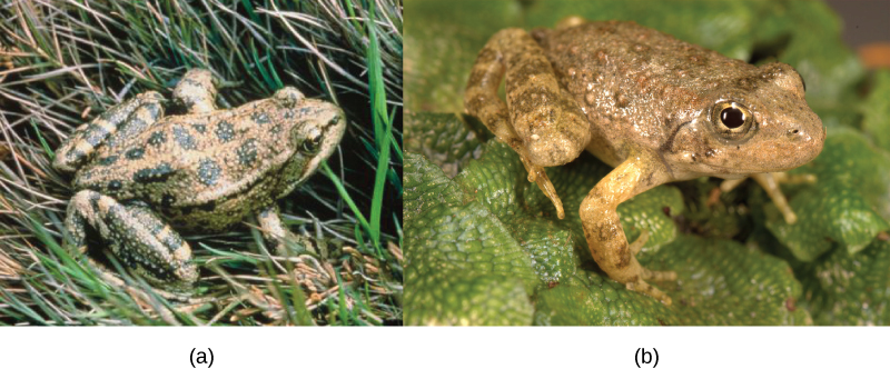
Photo a shows Rana aurora, a beige frog with green spots. Photo b shows Rana boylii, a brown frog.
Figure 18.17 — 18.2 Formation of New Species

Figure 18.17 These two related frog species exhibit temporal reproductive isolation. (a) Rana aurora breeds earlier in the year than (b) Rana boylii . (credit a: modification of work by Mark R. Jennings, USFWS; credit b: modification of work by Alessandro Catenazzi)

Mary Ann Clark, Matthew Douglas, and Jung Choi, Biology 2E, OpenStax. (credit a: modification of work by Mark R. Jennings, USFWS; credit b: modification of work by Alessandro Catenazzi) · CC BY-NC-SA 4.0 · Original image ↗ · Access for free ↗
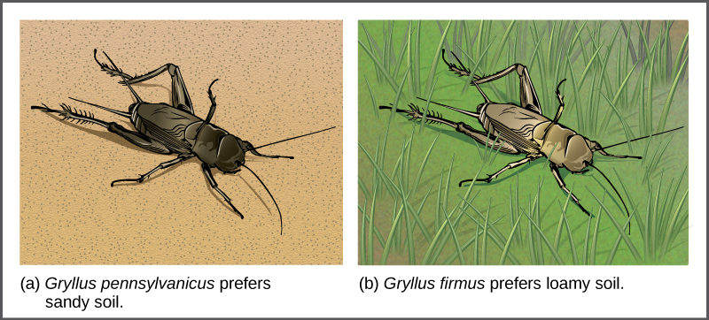
Illustration A shows the black Gryllus pennsylvanicus cricket on sandy soil, and illustration B shows the beige Gryllus firmus cricket in grass.
Figure 18.18 — 18.2 Formation of New Species

Figure 18.18 Speciation can occur when two populations occupy different habitats. The habitats need not be far apart. The cricket (a) Gryllus pennsylvanicus prefers sandy soil, and the cricket (b) Gryllus firmus prefers loamy soil. The two species can live in close proximity, but because of their different soil preferences, they became genetically isolated.

Mary Ann Clark, Matthew Douglas, and Jung Choi, Biology 2E, OpenStax. · CC BY-NC-SA 4.0 · Original image ↗ · Access for free ↗

Illustrations show four different types of damselfly reproductive organs. Each organ has a hook, but the shape and length of the hook varies, as does the shape of the organ itself.
Figure 18.19 — 18.2 Formation of New Species

Figure 18.19 The shape of the male reproductive organ varies among male damselfly species, and is only compatible with the female of that species. Reproductive organ incompatibility keeps the species reproductively isolated.

Mary Ann Clark, Matthew Douglas, and Jung Choi, Biology 2E, OpenStax. · CC BY-NC-SA 4.0 · Original image ↗ · Access for free ↗
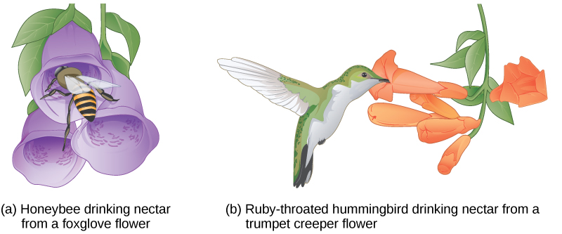
Illustration a shows a bee collecting pollen from a bright purple foxglove flower. The bee's body fits inside the bell like flower. Illustration B shows a hummingbird drinking nectar from a long tube like trumpet creeper flower.
Figure 18.20 — 18.2 Formation of New Species

Figure 18.20 Some flowers have evolved to attract certain pollinators. The (a) wide foxglove flower is adapted for pollination by bees, while the (b) long, tube-shaped trumpet creeper flower is adapted for pollination by hummingbirds.

Mary Ann Clark, Matthew Douglas, and Jung Choi, Biology 2E, OpenStax. · CC BY-NC-SA 4.0 · Original image ↗ · Access for free ↗
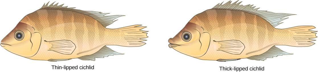
Illustrations show two species of cichlid fish which are similar in appearance except that one has thin lips, and one has thick lips.
Figure 18.21 — 18.2 Formation of New Species

Figure 18.21 Cichlid fish from Lake Apoyeque, Nicaragua, show evidence of sympatric speciation. Lake Apoyeque, a crater lake, is 1800 years old, but genetic evidence indicates that a single population of cichlid fish populated the lake only 100 years ago. Nevertheless, two populations with distinct morphologies and diets now exist in the lake, and scientists believe these populations may be in an early stage of speciation.

Mary Ann Clark, Matthew Douglas, and Jung Choi, Biology 2E, OpenStax. · CC BY-NC-SA 4.0 · Original image ↗ · Access for free ↗

Source: 18.2 Formation of New Species
209 terms, alphabetically ordered

Acid · ·

In the Brønsted–Lowry model, a substance that can donate a . Acidic have a higher activity than water.

Read explanation · OpenStax ↗
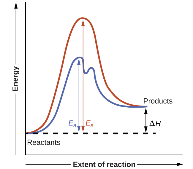
Activation energy ·

The energy barrier that must overcome to reach a and undergo .

Read explanation · OpenStax ↗
Active catalytic-site concentration ·

The total of active sites used to calculate from . It equals active when each has one site.

Read explanation · Biology LibreTexts ↗
Active site

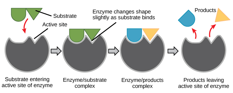
The region of an that binds its and carries out .

Read explanation · OpenStax ↗
adaptation

A heritable feature shaped by selection because it improves reproductive success in a relevant environment.

Read explanation · OpenStax ↗
Adenosine triphosphate

An energy-carrying ; its powers many cellular processes, including cycles.

Read explanation · OpenStax ↗
Allele

One version or copy of a at a ; a typical cell carries two copies of an autosomal .

Read explanation · NCBI Bookshelf / Sinauer Associates ↗
allele frequency

The proportion of copies of a specified represented by a particular .

Read explanation · OpenStax ↗
allopatric speciation

associated with geographic separation of populations.

Read explanation · OpenStax ↗
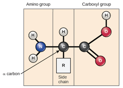
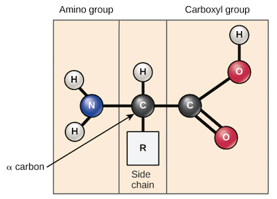
Alpha carbon · ·

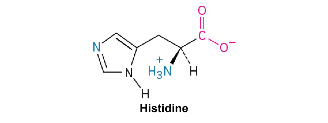
The central carbon next to the carboxyl carbon. In a standard it binds an , hydrogen, and .

Read explanation · OpenStax ↗
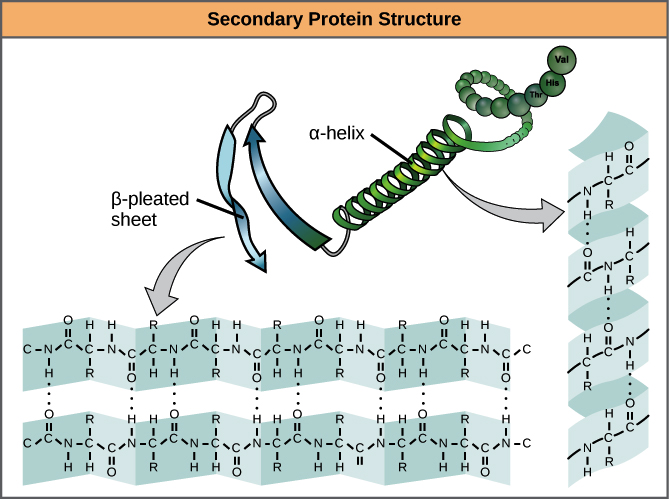
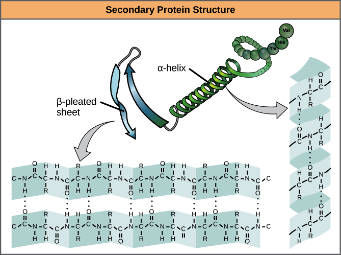
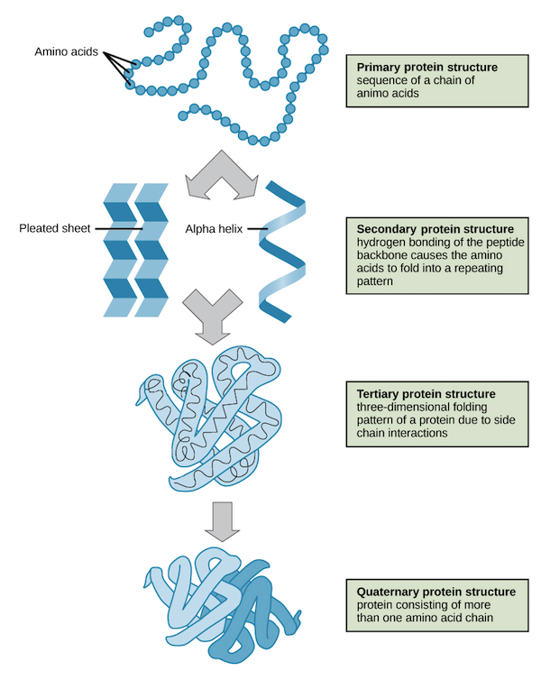
Alpha helix · · · · · ·

A helical stabilized by between a oxygen and an hydrogen four later.

Read explanation · OpenStax ↗
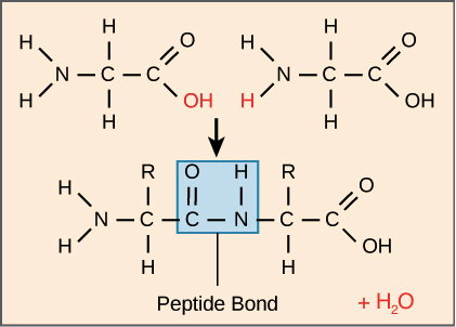
Amide · · ·

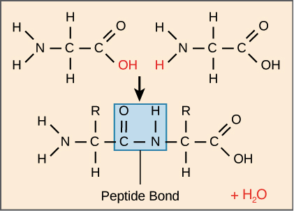
A group containing a carbon bonded to nitrogen. are amide linkages.

Read explanation · OpenStax ↗
Amino acid

A building block containing amino and and a characteristic .

Read explanation · OpenStax ↗
Amino acid residue · ·

The part of an incorporated into a chain. Residue can also describe another building block within a larger .

Read explanation · OpenStax ↗
Amino group · · ·

A nitrogen-containing . A free ’s amino group is typically (NH₃⁺) near physiological ; ’s ring nitrogen is an exception to this formula.

Read explanation · OpenStax ↗
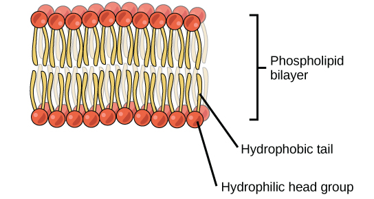
Amphipathic

Having both a region and a region, as in a or .

Read explanation · OpenStax ↗
Analytical standard ·

A material with a known identity or amount used to compare or calibrate measurements.

Read explanation · Agilent ↗
anemia

Reduced blood oxygen-carrying capacity associated with low or red-cell mass for the relevant reference context.

Read explanation · OpenStax ↗
Anticodon

A triplet that pairs to an . The anticodon for 5′-AUG-3′ is aligned 3′-UAC-5′, or written 5′-CAU-3′.

Read explanation · NCBI Bookshelf / Garland Science ↗
Antiparallel

Running in opposite directions, as with two strands or neighboring strands in some .

Read explanation · OpenStax ↗
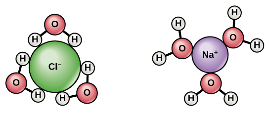
Aqueous solution ·

A in which water is the .

Read explanation · OpenStax ↗
Archaea ·

A of distinct from , with characteristic chemistry and -expression machinery.

Read explanation · OpenStax ↗
Aromatic

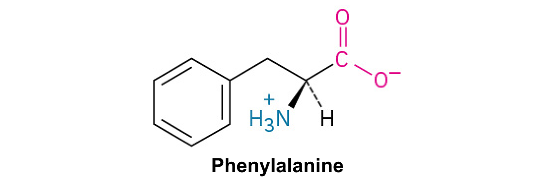
Containing a cyclic, with . , , and have aromatic .

Read explanation · OpenStax ↗
Atom

The smallest unit of an element that retains its chemical identity; it has a surrounded by .

Read explanation · OpenStax ↗
Bacteria ·

A of single-celled . Bacterial cells lack a -bound and are distinct from .

Read explanation · OpenStax ↗
Benzene ring

A six-carbon ring with .

Read explanation · OpenStax ↗
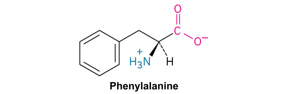
Benzyl group

A attached through a –CH₂– group; part of ’s .

Read explanation · OpenStax ↗
Beta sheet · · · · · ·

A made of aligned segments connected by ; strands may be parallel or .

Read explanation · OpenStax ↗
Biomolecule

A made by or involved in living systems, including , , , and .

Read explanation · OpenStax ↗
Blotting ·

Transfer of separated or to a so a specific target can be detected.

Read explanation · Thermo Fisher ↗
bottleneck

A sharp population that can randomly remove genetic diversity.

Read explanation · OpenStax ↗
Brønsted–Lowry base · · · · · · · · · · ·

In the Brønsted–Lowry model, a substance that can accept a . Basic solutions have lower activity than water.

Read explanation · OpenStax ↗
Calibration

Establishing the relation between a measured signal and known values or .

Read explanation · Agilent ↗
Cancer

A group of diseases involving abnormal cells that can proliferate without normal restraints and invade tissues.

Read explanation · OpenStax ↗
Carbohydrate

A class of including sugars and their , used for energy storage, structure, and recognition.

Read explanation · OpenStax ↗
Carbonyl group · ·

A carbon double-bonded to oxygen, C=O; present in and many other .

Read explanation · OpenStax ↗
Carboxyl group · ·

An , COOH. In free it is usually to COO⁻ near physiological .

Read explanation · OpenStax ↗
Catalyst · ·

A substance that speeds a by providing a pathway with lower and is regenerated rather than consumed overall.

Read explanation · OpenStax ↗
Chemical reaction ·

A process that rearranges and chemical bonds, converting into .

Read explanation · OpenStax ↗
chi-square statistic

A sum of squared observed-minus-expected differences divided by expected counts, used in suitable categorical-data tests.

Read explanation · OpenStax ↗
Chromatography

Separation of mixture components by their different interactions with a and a moving .

Read explanation · Waters ↗
Chromosome ·

An organized with associated that carries . A replicated chromosome has two .

Read explanation · OpenStax ↗
Codon

A sequence of three that specifies an or a stop signal.

Read explanation · OpenStax ↗
complete dominance

An inheritance relationship in which the specified matches one .

Read explanation · OpenStax ↗
Concentration

The amount of a substance in a specified volume or mass of mixture.

Read explanation · OpenStax ↗
Conjugated system ·

Adjacent orbitals that allow to be distributed across several , often through alternating single and multiple bonds.

Read explanation · OpenStax ↗
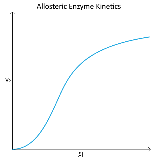
Cooperativity · ·

An interaction in which binding at one site changes binding at other sites. Positive cooperativity can produce a response.

Read explanation · Biology LibreTexts ↗
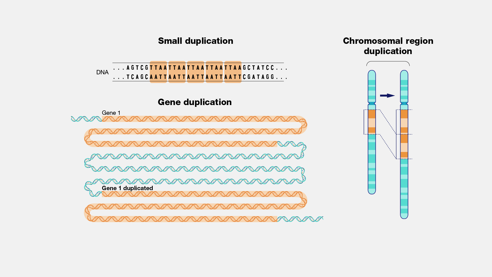
Copy number ·

The number of copies of a segment in a defined sample or ; it is distinct from or abundance.

Read explanation · NHGRI / NIH ↗
Covalent bond · ·

A bond in which share pairs. and are covalent.

Read explanation · OpenStax ↗
Cysteine ·

An with a . Two cysteines can form a .

Read explanation · OpenStax ↗
Deoxyribonucleic acid

The that stores genetic information used to specify and sequences.

Read explanation · OpenStax ↗
Deprotonation

Removal of a from a or group; this changes its by minus one.

Read explanation · OpenStax ↗
Detergent

An substance that can associate with both water and material; detergents can disrupt or interactions.

Read explanation · Thermo Fisher ↗
determination

Developmental commitment to a cell fate before all specialized features necessarily appear.

Read explanation · OpenStax ↗
Diploid

Having two sets; comparisons of must account for and sample composition.

Read explanation · NHGRI / NIH ↗
directional selection

Selection that favors one end of a trait distribution.

Read explanation · OpenStax ↗
disruptive selection

Selection that favors extremes over intermediate trait values.

Read explanation · OpenStax ↗
Disulfide bond · · ·

A covalent sulfur–sulfur bond formed by of two , which can stabilize structure.

Read explanation · NCBI Bookshelf ↗
DNA replication

Copying so genetic information can be passed to daughter cells. Each guides a complementary new strand.

Read explanation · OpenStax ↗
dominant

Describing an whose specified is expressed in a ; dominance does not imply greater frequency or .

Read explanation · OpenStax ↗
Electric charge · · ·

An electrical property that can be positive or negative. Opposite charges attract and like charges repel; net charge is the sum of all charges on a particle.

Read explanation · OpenStax ↗
Electron

A negatively subatomic particle. Electron sharing and transfer determine much of chemical bonding.

Read explanation · OpenStax ↗
Electron delocalization ·

Distribution of across several rather than confinement to one or bond.

Read explanation · OpenStax ↗
Electronegativity ·

An ’s tendency to attract shared in a chemical bond. Unequal attraction can make a bond .

Read explanation · OpenStax ↗
Enzyme

A biological that speeds a without being consumed. Most enzymes are .

Read explanation · OpenStax ↗
Enzyme saturation · ·

The high- limit in which sites spend almost all their time processing and the rate approaches .

Read explanation · Biology LibreTexts ↗
Equilibrium

A state where opposing processes occur at equal rates, so macroscopic or other properties remain constant.

Read explanation · OpenStax ↗
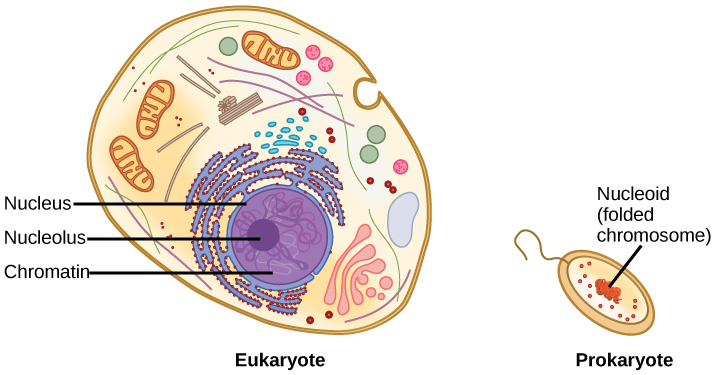
Eukaryote ·

An organism whose cells have a -enclosed ; animals, plants, fungi, and protists are eukaryotes.

Read explanation · OpenStax ↗
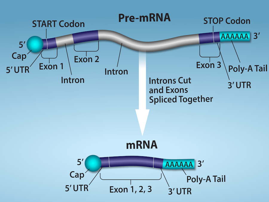
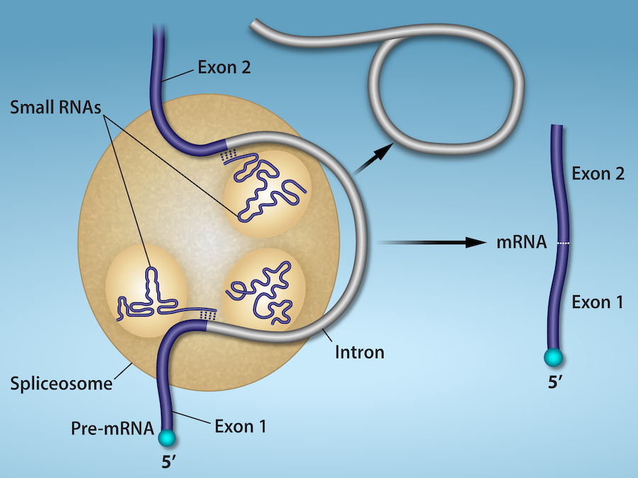
Exon

A segment retained in a mature spliced . In an exon may contain coding sequence, untranslated sequence, or both.

Read explanation · OpenStax ↗
Experimental control ·

A comparison sample or condition used to distinguish the effect being tested from other influences.

Read explanation · Thermo Fisher ↗
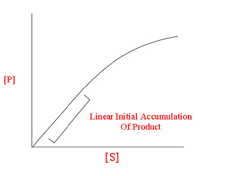
First-order kinetics

A rate dependence proportional to the first power of a . At low , a is approximately first-order in .

Read explanation · Biology LibreTexts ↗
fitness

Relative reproductive contribution of a or organism in a particular environment.

Read explanation · OpenStax ↗
founder effect

Altered when a new population starts from a small sample of a larger one.

Read explanation · OpenStax ↗
Fraction · ·

A portion of a sample collected during a separation, such as the fluid leaving a column during a time interval.

Read explanation · Waters ↗
frequency-dependent selection

Selection in which a variant’s depends on its frequency in the population.

Read explanation · OpenStax ↗
Functional group

A group of whose chemical behavior gives a characteristic and properties.

Read explanation · OpenStax ↗
gamete

A reproductive cell that contributes a during fertilization.

Read explanation · OpenStax ↗
Gene

A sequence that contributes to a functional or , together with the information needed to express it.

Read explanation · OpenStax ↗
Gene expression

Production of a functional from a , including and, for -coding , .

Read explanation · NCBI Bookshelf ↗
gene flow

Movement of between populations through successful reproduction by migrants or transferred .

Read explanation · OpenStax ↗
Genetic code

The correspondence between and or termination signals used during .

Read explanation · OpenStax ↗
genetic drift

Random changes in caused by finite sampling across generations.

Read explanation · OpenStax ↗
Genome

The complete genetic material of an organism or cell.

Read explanation · OpenStax ↗
genotype

The allelic composition of an organism at one or more specified .

Read explanation · OpenStax ↗
Gradient

A change in a quantity, such as , , or density, across a distance or over time.

Read explanation · Thermo Fisher ↗
Half-life

The time required for half of a population or amount to remain during decay; a constant half-life is characteristic of decay.

Read explanation · OpenStax ↗
Haploid

Having one set of , as in a human .

Read explanation · OpenStax ↗
Hardy–Weinberg equilibrium ·

A population null model with frequencies p², 2pq, and q² under random mating and other stated assumptions.

Read explanation · OpenStax ↗
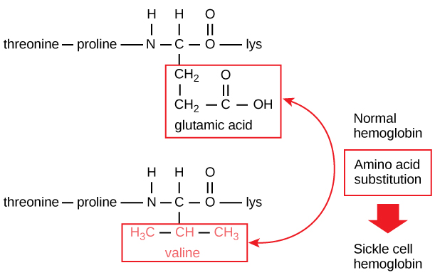
Hemoglobin

The oxygen-carrying in , composed of four with heme groups.

Read explanation · OpenStax ↗
heritability

Proportion of observed variation associated with genetic variation in a specified population and environment.

Read explanation · OpenStax ↗
heterozygote ·

An individual with two different at a specified .

Read explanation · OpenStax ↗
Histidine ·

A with an . Mostly uncharged near physiological , it can accept or donate .

Read explanation · OpenStax ↗
homozygote ·

An individual with two identical at a specified .

Read explanation · OpenStax ↗
Hybridization

Pairing of complementary strands, used for sequence-specific detection.

Read explanation · NHGRI ↗
Hydrogen bond ·

An attraction between a hydrogen bonded to an and another . hydrogen bonds stabilize .

Read explanation · OpenStax ↗
Hydrogen ion · ·

A positively hydrogen species. H⁺ denotes a , which is hydrated in water; its activity determines .

Read explanation · OpenStax ↗
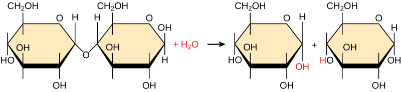
Hydrolysis

Breaking a chemical bond by adding water. hydrolysis separates .

Read explanation · OpenStax ↗
Hydrophilic

Interacting favorably with water, typically because a group is or .

Read explanation · OpenStax ↗
Hydrophobic

Interacting poorly with water. often gather in a ’s interior.

Read explanation · OpenStax ↗
Hydroxide ion ·

The negatively OH⁻. Basic contain a higher hydroxide ion activity than water at the same temperature.

Read explanation · OpenStax ↗
Hydroxyl group ·

An oxygen bonded to hydrogen, –OH. Hydroxyl groups can and often increase .

Read explanation · OpenStax ↗
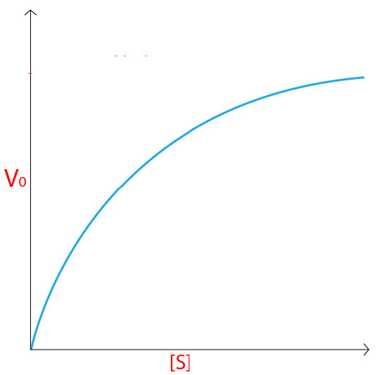
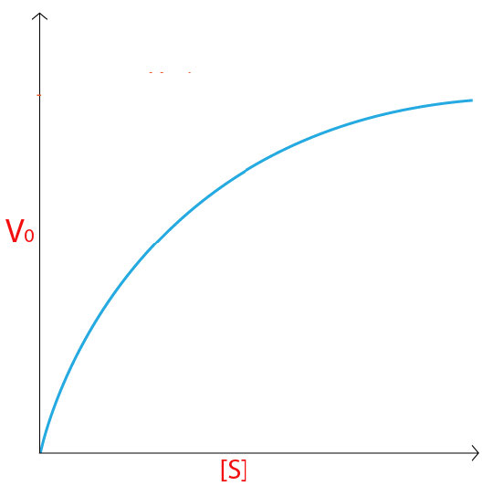
Hyperbolic curve ·

A curve that approaches an asymptote. The standard rate curve is a rectangular hyperbola approaching .

Read explanation · Biology LibreTexts ↗
Imidazole

A five-membered ring containing two nitrogens; ’s contains this ring.

Read explanation · OpenStax ↗
inbreeding

Mating among relatives, increasing relative to random mating without necessarily changing directly.

Read explanation · OpenStax ↗
inclusive fitness

Reproductive effects through an individual’s own offspring and effects on relatives weighted by genetic relatedness.

Read explanation · OpenStax ↗
Indole

A fused six-membered and five-membered ring system containing nitrogen; found in .

Read explanation · OpenStax ↗
Initial reaction rate · · · ·

The early rate of formation, measured before substantial depletion or accumulation, usually after the brief binding transient.

Read explanation · Biology LibreTexts ↗
Intron ·

A segment removed from a precursor during . Intronic signals or regulatory sequences can affect .

Read explanation · OpenStax ↗
Ion · ·

An or with a net because its numbers of and do not balance.

Read explanation · OpenStax ↗
linkage

A tendency of nearby on the same to be inherited together.

Read explanation · OpenStax ↗
Lipid

A broad class of largely or , including fats, , and steroids.

Read explanation · OpenStax ↗
locus

The specific position of a or other feature.

Read explanation · OpenStax ↗
Logarithm · · ·

The exponent needed to obtain a number from a chosen fixed number. For decimal logarithms, log₁₀(100) = 2 because 10² = 100; uses the negative decimal logarithm of activity.

Read explanation · OpenStax ↗
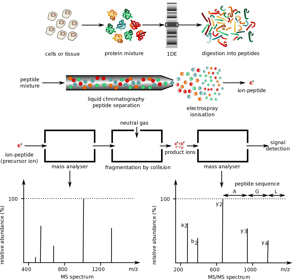
Mass spectrometry ·

Analysis of according to their mass-to- ratios, used to identify and or .

Read explanation · Thermo Fisher ↗
Mass-to-charge ratio

The mass of an divided by its number; this is the quantity measured by a .

Read explanation · Thermo Fisher ↗
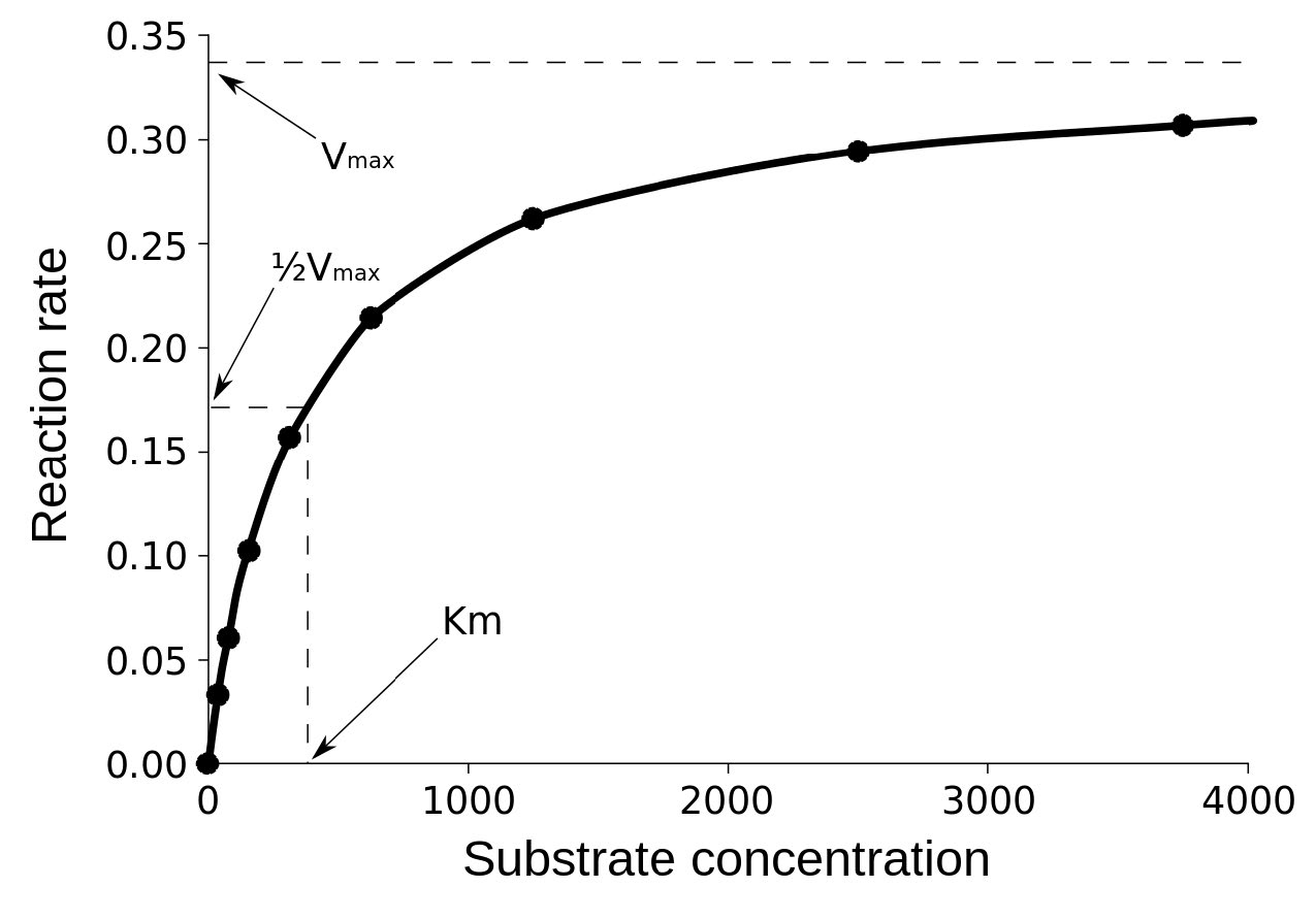
Maximum reaction rate · ·

The limiting as becomes saturating. For a fixed under given conditions, Vmax = times .

Read explanation · Biology LibreTexts ↗
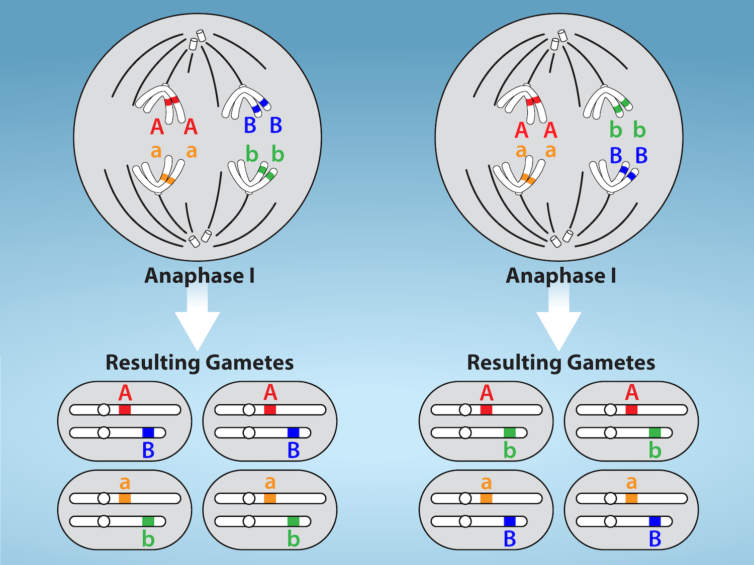
meiosis

Two successive divisions after one that usually produce cells from a precursor.

Read explanation · OpenStax ↗
Membrane · · · ·

A thin boundary or sheet. Cell membranes are bilayers containing ; membranes are synthetic supports that hold or for detection.

Read explanation · OpenStax ↗
Messenger RNA ·

An that carries coding information used by to synthesize a .

Read explanation · OpenStax ↗
Metabolism

The chemical that build , break them down, and transform energy in a living system.

Read explanation · OpenStax ↗
Michaelis–Menten kinetics · ·

A model with = [S]/(Km + ). Its curve is ; may require a different model.

Read explanation · Biology LibreTexts ↗
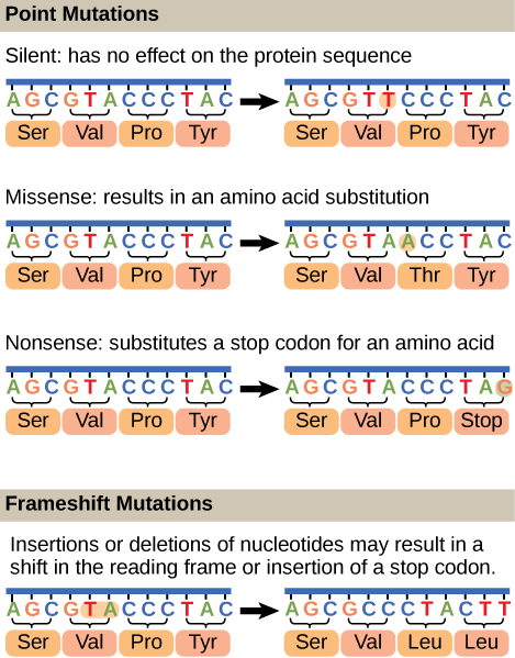
Missense mutation ·

A coding-sequence that changes the specified ; its effect depends on the and context.

Read explanation · OpenStax ↗
Mobile phase

The moving fluid that carries a sample through a system.

Read explanation · Waters ↗
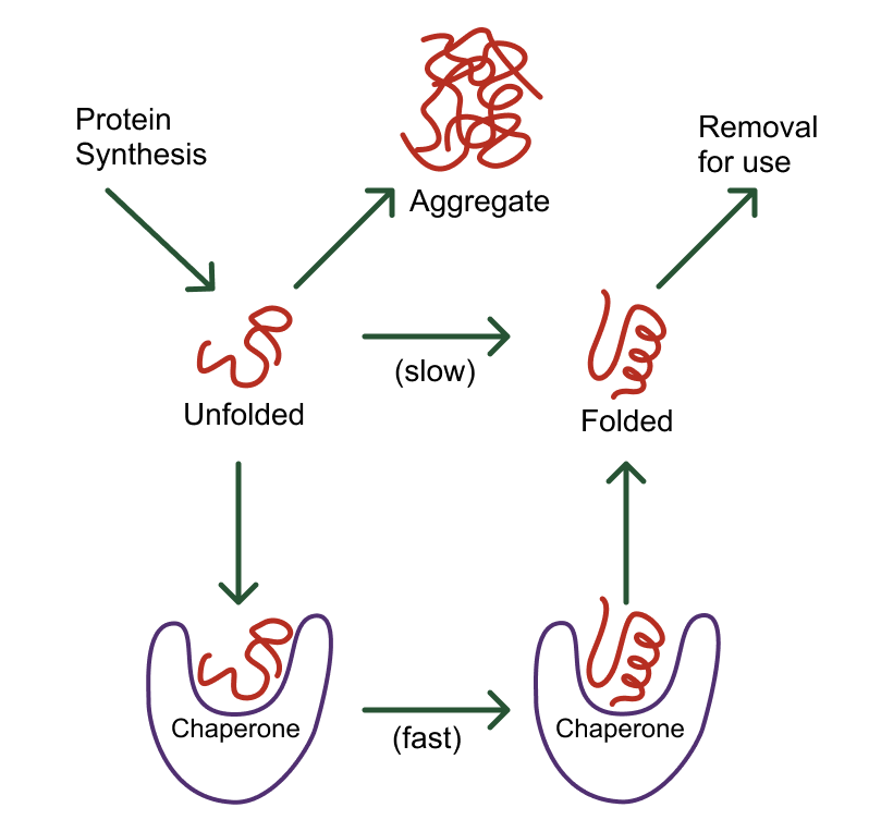
Molecular chaperone · ·

A that assists other in folding or prevents , without specifying their sequence.

Read explanation · NCBI Bookshelf ↗
Molecule

Two or more joined by . A molecule may be electrically or carry a .

Read explanation · OpenStax ↗
Mutation

A change in a sequence; some mutations alter a ’s sequence.

Read explanation · OpenStax ↗
natural selection

Differential reproductive success associated with heritable variation.

Read explanation · OpenStax ↗
Neutral

Having no net . For a , neutral instead means equal and activities; its is about 7 at 25 °C.

Read explanation · OpenStax ↗
Nitrogenous base · · ·

A nitrogen-containing ring component of ; its pairing interactions help specify sequences.

Read explanation · OpenStax ↗
Nonpolar ·

Lacking a substantial separation of . Nonpolar groups generally interact poorly with water.

Read explanation · OpenStax ↗
Nonsense mutation ·

A that converts an amino- into a premature , potentially truncating the or destabilizing its .

Read explanation · OpenStax ↗
Nucleic acid

A of , such as or , used in information storage, expression, and other cellular functions.

Read explanation · OpenStax ↗
Nucleotide

A joined to a sugar and one or more .

Read explanation · OpenStax ↗
Nucleus ·

A -enclosed compartment containing most of a cell’s .

Read explanation · OpenStax ↗
outbreeding

Mating among less-related individuals or populations, often increasing .

Read explanation · OpenStax ↗
Oxidation ·

Loss of or an increase in oxidation state. Oxidizing two can form a .

Read explanation · OpenStax ↗
p value

The probability, under a specified null model, of data at least as incompatible with that model as those observed.

Read explanation · OpenStax ↗
Peptide

A chain of joined by ; the term commonly describes chains shorter than a typical .

Read explanation · OpenStax ↗
Peptide bond ·

A covalent between the carboxyl carbon of one and the amino nitrogen of the next.

Read explanation · OpenStax ↗
pH

A measure of , defined as the negative of activity. Lower pH means greater ; pH influences .

Read explanation · OpenStax ↗
phenotype

A measurable trait produced by interacting with development and environment.

Read explanation · OpenStax ↗
Phenylalanine ·

A with an .

Read explanation · OpenStax ↗
Phosphate group ·

A phosphorus-containing group bonded to oxygens; phosphate groups occur in , , and modified .

Read explanation · OpenStax ↗
Phospholipid

An with a -containing region and tails; a major component of cellular .

Read explanation · OpenStax ↗
photon

Quantum of electromagnetic radiation with energy hf.

Read explanation · OpenStax ↗
ploidy

The number of complete sets in a cell.

Read explanation · OpenStax ↗
Polar

Having an uneven distribution of . Polar groups often interact favorably with water.

Read explanation · OpenStax ↗
Polymer

A large made from many linked molecular building blocks.

Read explanation · OpenStax ↗
polymorphism

Coexistence of multiple genetic variants or in a population.

Read explanation · OpenStax ↗
Polypeptide

A chain of connected by . A functional can contain one or several such chains.

Read explanation · OpenStax ↗
polyploidy

Possession of more than two complete sets.

Read explanation · OpenStax ↗
population stratification

Population substructure that can confound genetic associations when ancestry relates to both and outcomes.

Read explanation · OpenStax ↗
postzygotic barrier

A reproductive barrier that reduces hybrid survival or reproduction after fertilization.

Read explanation · OpenStax ↗
prezygotic barrier

A reproductive barrier that prevents mating or fertilization.

Read explanation · OpenStax ↗
Prokaryote ·

An organism whose cells lack a -bound ; and are prokaryotes.

Read explanation · OpenStax ↗
Proline ·

An whose loops back to the nitrogen, restricting rotation and often creating bends.

Read explanation · OpenStax ↗
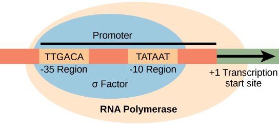
Promoter

A region that recruits machinery and helps specify where and in which direction begins.

Read explanation · OpenStax ↗
Protein

One or more folded chains that perform biological roles such as , transport, signaling, or structural support.

Read explanation · OpenStax ↗
Protein aggregation · ·

Association of into larger clusters, often when exposed surfaces of unfolded stick together.

Read explanation · NCBI Bookshelf ↗
Protein backbone ·

The repeating nitrogen–alpha-carbon– chain of a , excluding its variable .

Read explanation · OpenStax ↗
Protein domain · ·

A region of a that forms a recognizable structural or functional unit.

Read explanation · OpenStax ↗
Proton

A positively subatomic particle. In – chemistry, donating a proton means transferring a .

Read explanation · OpenStax ↗
Protonation

Addition of a to an , , or ; this changes its by plus one.

Read explanation · OpenStax ↗
Quantification · ·

Estimating the amount or of a substance from measured signals and suitable or .

Read explanation · Waters ↗
R group · ·

The variable side chain attached to an ’s . It determines identity, , , and chemical behavior.

Read explanation · OpenStax ↗
Reactant

A starting substance transformed during a .

Read explanation · OpenStax ↗
Reaction intermediate · ·

A species formed in one step and consumed in another. It occupies a local energy minimum between .

Read explanation · OpenStax ↗
Reaction product ·

A substance formed by a .

Read explanation · OpenStax ↗
reaction quotient

-to- activity ratio with stoichiometric exponents at the current composition.

Read explanation · OpenStax ↗
Reaction rate · ·

How quickly are consumed or form, usually expressed as a change per unit time.

Read explanation · OpenStax ↗
recessive

Describing an whose specified is masked by another in a .

Read explanation · OpenStax ↗
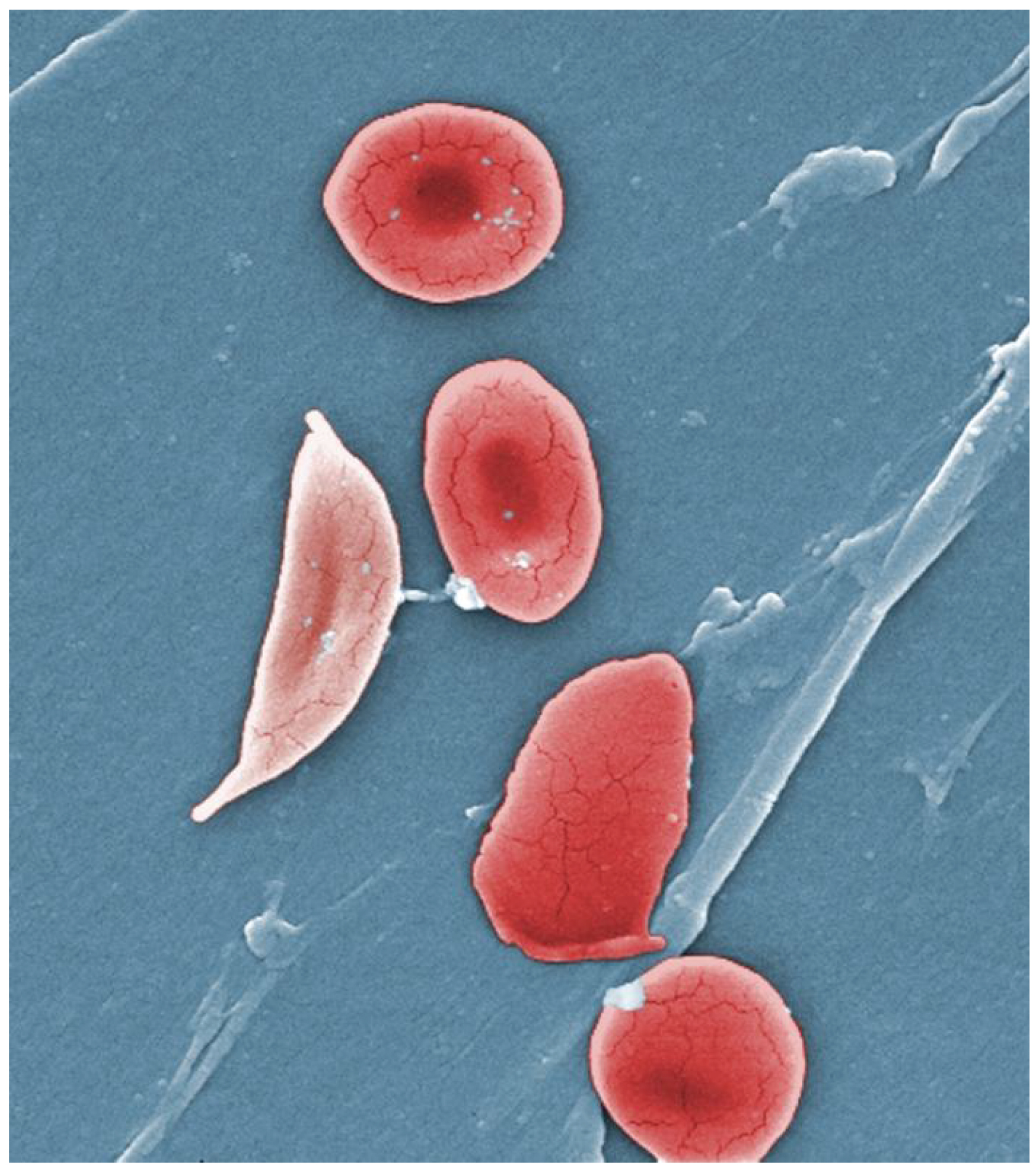
Red blood cell · ·

A blood cell that transports oxygen using ; mature human red blood cells lack a .

Read explanation · OpenStax ↗
Reduction

Gain of or a decrease in state. Reducing a restores two .

Read explanation · OpenStax ↗
Release factor ·

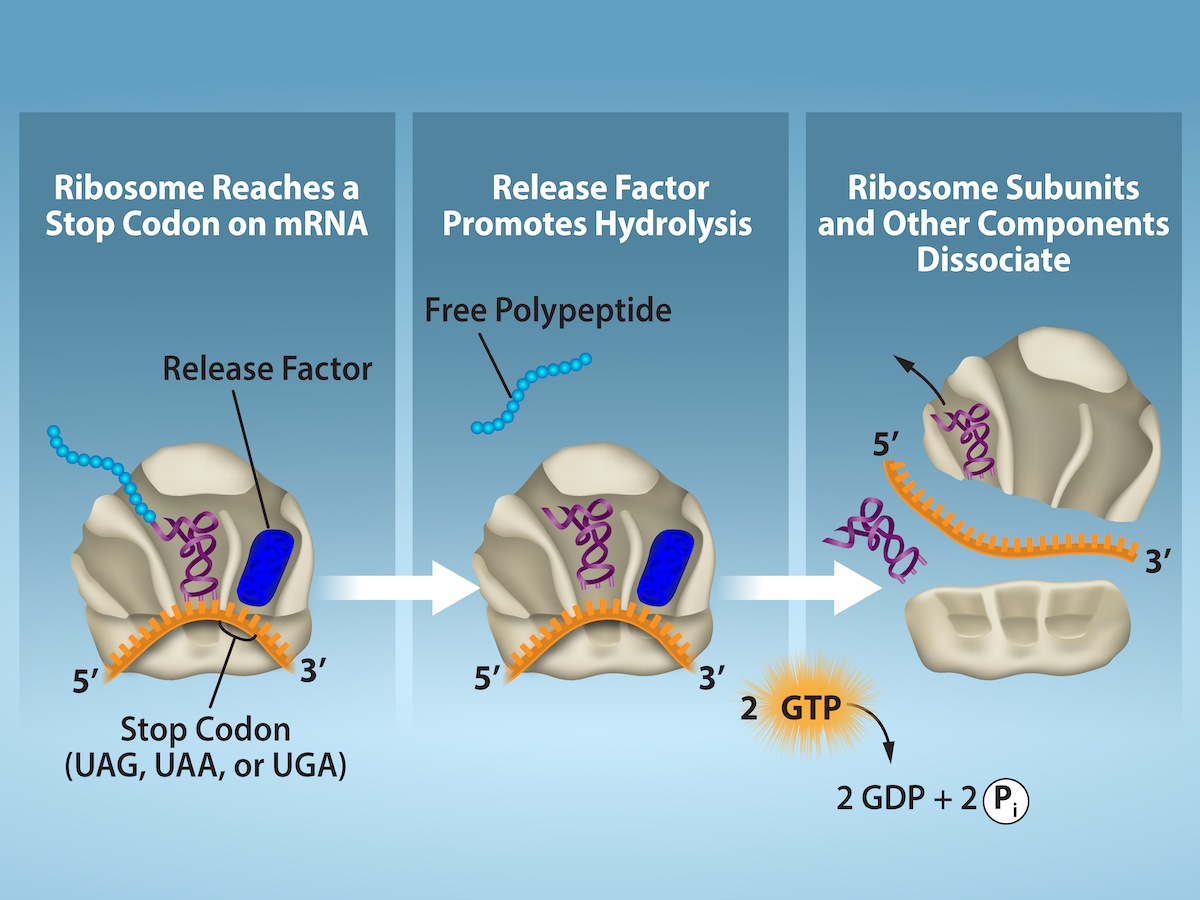
A that recognizes a stop signal and promotes of the – to release the .

Read explanation · OpenStax ↗
Ribonucleic acid ·

A with roles in , regulation, and ; carries -coding information.

Read explanation · OpenStax ↗
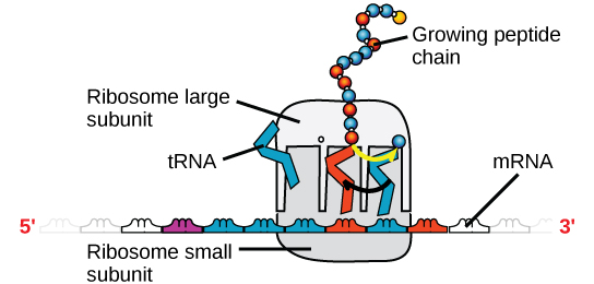
Ribosome ·

A complex of and that translates into a .

Read explanation · OpenStax ↗
RNA splicing · ·

Removal of and joining of in a precursor .

Read explanation · NCBI Bookshelf / Garland Science ↗
RNA stability

Persistence of an before degradation; greater stability generally means a longer lifetime or under specified conditions.

Read explanation · OpenStax ↗
Secondary structure

Local folding, such as and , stabilized mainly by .

Read explanation · OpenStax ↗
shaping

Reinforcing successive approximations toward a target behavior.

Read explanation · OpenStax ↗
Sigma factor · · ·

A -polymerase-associated factor that helps recognize sequences and initiate .

Read explanation · OpenStax ↗
Sigmoidal curve ·

An S-shaped curve. A sigmoidal rate-versus- curve can indicate rather than simple behavior.

Read explanation · Biology LibreTexts ↗
Sister chromatid

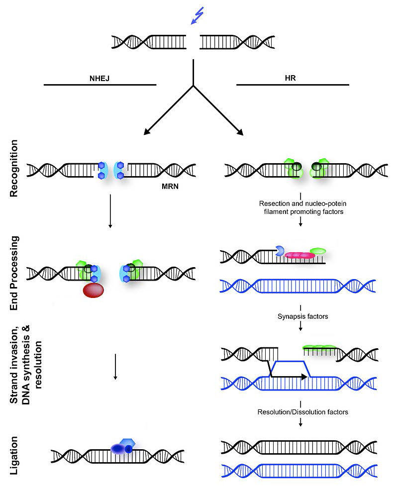
One of the two copies of a produced by . An intact sister chromatid can supply a template for accurate repair.

Read explanation · Biology LibreTexts / Oregon State University ↗
Solubility ·

The amount of a substance that can dissolve in a under specified conditions. Soluble means able to dissolve; insoluble means only very slightly soluble in that .

Read explanation · OpenStax ↗
Solute

A dissolved component of a .

Read explanation · OpenStax ↗
Solution

A homogeneous mixture in which are dissolved in a .

Read explanation · OpenStax ↗
Solvent

The component of a that dissolves other substances, usually the component present in the greatest amount.

Read explanation · OpenStax ↗
speciation

Evolutionary divergence that establishes distinct species, often through reproductive isolation.

Read explanation · OpenStax ↗
Spectrum ·

A distribution of measured signal over a variable such as or .

Read explanation · Thermo Fisher ↗
stabilizing selection

Selection that favors intermediate values of a trait.

Read explanation · OpenStax ↗
Stationary phase

The material that remains fixed in a system.

Read explanation · Waters ↗
Stop codon · · ·

An that recruits a to end : UAA, UAG, or UGA in the standard code.

Read explanation · OpenStax ↗
Substitution · ·

Replacement of one by another. In a coding region it can be , , or .

Read explanation · OpenStax ↗
Substrate

A that an binds and chemically transforms.

Read explanation · OpenStax ↗
Substrate concentration

The amount of per volume. Square brackets denote ; [S] is varied to measure an curve.

Read explanation · Biology LibreTexts ↗
Subunit ·

An individual chain within a containing multiple chains.

Read explanation · OpenStax ↗
sympatric speciation

without an initial geographic barrier separating populations.

Read explanation · OpenStax ↗
Synonymous mutation · · · · ·

A coding-sequence that leaves the specified unchanged. It can still affect , , or .

Read explanation · OpenStax ↗
Template strand · · ·

A preexisting strand whose sequence guides complementary nucleic- synthesis.

Read explanation · OpenStax ↗
Thiol group · · · ·

A sulfur bonded to hydrogen, –SH. thiols can form through .

Read explanation · OpenStax ↗
Transcription

Synthesis of using a template.

Read explanation · OpenStax ↗
Transfer RNA ·

An adaptor that carries an and pairs its with a on .

Read explanation · OpenStax ↗
Transition state

A fleeting, high-energy arrangement at a barrier. It is an energy maximum along the path, rather than a stable .

Read explanation · OpenStax ↗
Translation ·

Synthesis of a on a using the sequence of in .

Read explanation · OpenStax ↗
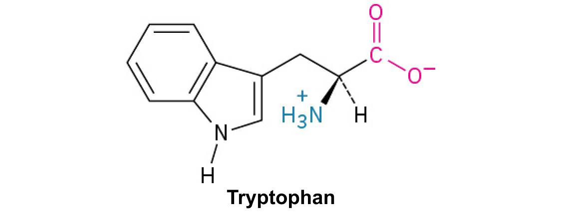
Tryptophan ·

An with a bulky ; commonly grouped as .

Read explanation · OpenStax ↗
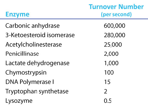
Turnover number · · ·

The maximum number of cycles per per unit time, calculated as /. Units are inverse time, commonly s⁻¹.

Read explanation · IUBMB ↗
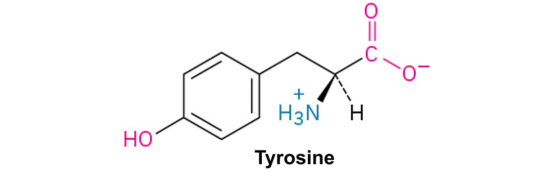
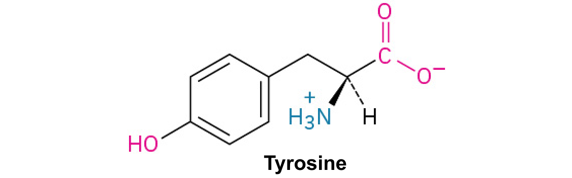
Tyrosine ·

An with a phenolic . Usually uncharged near physiological .

Read explanation · OpenStax ↗
Wavelength

The distance between repeating points of a wave, such as neighboring crests; light wavelength determines energy.

Read explanation · JASCO ↗
zygote

The single cell formed by fusion and union of parental genetic contributions.

Read explanation · OpenStax ↗

19.1 Population Evolution

OpenStax · 19.1 Population Evolution ↗
Instructional page including learning objectives, examples, figures, source tables and questions. Site navigation and embedded media players are omitted; source media links remain available.

Learning Objectives

By the end of this section, you will be able to do the following:

  • Define population genetics and describe how scientists use population genetics in studying population evolution
  • Define the Hardy-Weinberg principle and discuss its importance

People did not understand the mechanisms of inheritance, or genetics, at the time Charles Darwin and Alfred Russel Wallace were developing their idea of . This lack of knowledge was a stumbling block to understanding many aspects of evolution. The predominant (and incorrect) genetic theory of the time, blending inheritance, made it difficult to understand how might operate. Darwin and Wallace were unaware of the Austrian monk Gregor Mendel's 1866 publication "Experiments in Plant ", which came out not long after Darwin's book, On the Origin of Species. Scholars rediscovered Mendel’s work in the early twentieth century at which time geneticists were rapidly coming to an understanding of the basics of inheritance. Initially, the newly discovered particulate nature of made it difficult for biologists to understand how gradual evolution could occur. However, over the next few decades scientists integrated genetics and evolution in what became known as the modern synthesis—the coherent understanding of the relationship between and genetics that took shape by the 1940s. Generally, this concept is accepted today. In short, the modern synthesis describes how evolutionary processes, such as , can affect a population’s genetic makeup, and, in turn, how this can result in the gradual evolution of populations and species. The theory also connects population change over time (microevolution), with the processes that gave rise to new species and higher taxonomic groups with widely divergent characters (macroevolution).

Everyday Connection

Evolution and Flu Vaccines

Every fall, the media starts reporting on flu vaccinations and potential outbreaks. Scientists, health experts, and institutions determine recommendations for different parts of the population, predict optimal production and inoculation schedules, create vaccines, and set up clinics to provide inoculations. You may think of the annual flu shot as media hype, an important health protection, or just a briefly uncomfortable prick in your arm. However, do you think of it in terms of evolution?

The media hype of annual flu shots is scientifically grounded in our understanding of evolution. Each year, scientists across the globe strive to predict the flu strains that they anticipate as most widespread and harmful in the coming year. They this knowledge on how flu strains have evolved over time and over the past few flu seasons. Scientists then work to create the most effective vaccine to combat those selected strains. Pharmaceutical companies produce hundreds of millions of doses in a short period in order to provide vaccinations to key populations at the optimal time.

Because viruses, like the flu, evolve very quickly (especially in evolutionary time), this poses quite a challenge. Viruses mutate and replicate at a fast rate, so the vaccine developed to protect against last year’s flu strain may not provide the protection one needs against the coming year’s strain. Evolution of these viruses means continued to ensure survival, including to survive previous vaccines.

Population Genetics

Recall that a for a particular character may have several , or variants, that code for different traits associated with that character. For example, in the ABO blood type system in humans, three determine the particular blood-type on the surface of . Each individual in a population of organisms can only carry two for a particular , but more than two may be present in the individuals that comprise the population. Mendel followed as they were inherited from parent to offspring. In the early twentieth century, biologists in the area of population genetics began to study how selective forces change a population through changes in and genotypic frequencies.

The (or frequency) is the rate at which a specific appears within a population. Until now we have discussed evolution as a change in the characteristics of a population of organisms, but behind that phenotypic change is genetic change. In population genetics, scientists define the term evolution as a change in the 's frequency in a population. Using the ABO blood type system as an example, the frequency of one of the , IA, is the number of copies of that divided by all the copies of the ABO in the population. For example, a study in Jordan1 found a frequency of IA to be 26.1 percent. The IB and I0 comprise 13.4 percent and 60.5 percent of the respectively, and all of the frequencies added up to 100 percent. A change in this frequency over time would constitute evolution in the population.

The within a given population can change depending on environmental factors; therefore, certain become more widespread than others during the process. can alter the population’s genetic makeup. An example is if a given confers a that allows an individual to better survive or have more offspring. Because many of those offspring will also carry the beneficial , and often the corresponding , they will have more offspring of their own that also carry the , thus, perpetuating the cycle. Over time, the will spread throughout the population. Some will quickly become fixed in this way, meaning that every individual of the population will carry the , while detrimental may be swiftly eliminated if derived from a from the pool. The pool is the sum of all the in a population.

Sometimes, within a population change randomly with no advantage to the population over existing . We call this phenomenon . and usually occur simultaneously in populations and are not isolated events. It is hard to determine which process dominates because it is often nearly impossible to determine the cause of change in at each occurrence. We call an event that initiates an change in an isolated part of the population, which is not typical of the original population, the . , random drift, and founder effects can lead to significant changes in a population's .

Hardy-Weinberg Principle of

In the early twentieth century, English mathematician Godfrey Hardy and German physician Wilhelm Weinberg stated the principle of to describe the population's genetic makeup. The theory, which later became known as the Hardy-Weinberg principle of , states that a population’s and frequencies are inherently stable—unless some kind of evolutionary force is acting upon the population, neither the nor the genotypic frequencies would change. The Hardy-Weinberg principle assumes an infinitely large population and conditions with no , migration, emigration, or selective pressure for or against . While no population can satisfy those conditions, the principle offers a useful model against which to compare real population changes.

Working under this theory, population geneticists represent different as different variables in their mathematical models. The variable p, for example, often represents the frequency of a particular , say Y for the trait of yellow in Mendel’s peas, while the variable represents the frequency of y that confer the color green. If these are the only two possible for a given in the population, p + = 1. In other words, all the p and all the comprise all of the for that in the population.

However, what ultimately interests most biologists is not the frequencies of different , but the frequencies of the resulting , known as the population’s genetic structure, from which scientists can surmise distribution. If we observe the , we can know only the 's . The calculations provide an estimate of the remaining . Since each individual carries two per , if we know the (p and ), predicting the ' frequencies is a simple mathematical calculation to determine the probability of obtaining these if we draw two at random from the pool. In the above scenario, an individual pea plant could be pp (YY), and thus produce yellow peas; pq (Yy), also yellow; or qq (yy), and thus produce green peas (Figure 19.2). In other words, the frequency of pp individuals is simply p2; the frequency of pq individuals is 2pq; and the frequency of qq individuals is 2. Again, if p and are the only two possible for a given trait in the population, these frequencies will sum to one: p2 + 2pq + 2 = 1.

Visual Connection

The Hardy-Weinberg principle is used to predict the genotypic distribution of offspring in a given population. In the example given, pea plants have two different alleles for pea color. The dominant capital Y allele results in yellow pea color, and the recessive small y allele results in green pea color. The distribution of individuals in a population of 500 is given. Of the 500 individuals, 245 are homozygous dominant (capital Y capital Y) and produce yellow peas. 210 are heterozygous (capital Y small y) and also produce yellow peas. 45 are homozygous recessive (small y small y) and produce green peas. The frequencies of homozygous dominant, heterozygous, and homozygous recessive individuals are 0.49, 0.42, and 0.09, respectively. Each of the 500 individuals provides two alleles to the gene pool, or 1000 total. The 245 homozygous dominant individuals provide two capital Y alleles to the gene pool, or 490 total. The 210 heterozygous individuals provide 210 capital Y and 210 small y alleles to the gene pool. The 45 homozygous recessive individuals provide two small y alleles to the gene pool, or 90 total. The number of capital Y alleles is 490 from homozygous dominant individuals plus 210 from homozygous recessive individuals, or 700 total. The number of small y alleles is 210 from heterozygous individuals plus 90 from homozygous recessive individuals, or 300 total. The allelic frequency is calculated by dividing the number of each allele by the total number of alleles in the gene pool. For the capital Y allele, the allelic frequency is 700 divided by 1000, or 0.7; this allelic frequency is called p. For the small y allele the allelic frequency is 300 divided by 1000, or 0.3; the allelic frequency is called q. Hardy-Weinberg analysis is used to determine the genotypic frequency in the offspring. The Hardy-Wienberg equation is p-squared plus 2pq plus q-squared equals 1. For the population given, the frequency is 0.7-squared plus 2 times .7 times .3 plus .3-squared equals one. The value for p-squared, 0.49, is the predicted frequency of homozygous dominant (capital Y capital Y) individuals. The value for 2pq, 0.42, is the predicted frequency of heterozygous (capital Y small y) individuals. The value for q-squared, .09, is the predicted frequency of homozygous recessive individuals. Note that the predicted frequency of genotypes in the offspring is the same as the frequency of genotypes in the parent population. If all the genotypic frequencies, .49 plus .42 plus .09, are added together, the result is one.
Figure 19.2 — 19.1 Population Evolution

Figure 19.2 When populations are in the Hardy-Weinberg equilibrium, the allelic frequency is stable from generation to generation and we can determine the allele distribution from the Hardy-Weinberg equation. If the allelic frequency measured in the field differs from the predicted value, scientists can make inferences about what evolutionary forces are at play.

Mary Ann Clark, Matthew Douglas, and Jung Choi, Biology 2E, OpenStax. · CC BY-NC-SA 4.0 · Original image ↗ · Access for free ↗

In plants, violet flower color (V) is over white (v). If p = 0.8 and = 0.2 in a population of 500 plants, how many individuals would you expect to be (VV), (Vv), and (vv)? How many plants would you expect to have violet flowers, and how many would have white flowers?

In theory, if a population is at —that is, there are no evolutionary forces acting upon it—generation after generation would have the same pool and genetic structure, and these equations would all hold true all of the time. Of course, even Hardy and Weinberg recognized that no natural population is immune to evolution. Populations in nature are constantly changing in genetic makeup due to drift, , possibly migration, and selection. As a result, the only way to determine the exact distribution of in a population is to go out and count them. However, the Hardy-Weinberg principle gives scientists a mathematical baseline of a non-evolving population to which they can compare evolving populations and thereby infer what evolutionary forces might be at play. If the frequencies of or deviate from the value expected from the Hardy-Weinberg equation, then the population is evolving.

Link to Learning

Use this online calculator to determine a population's genetic structure.

19.2 Population Genetics

OpenStax · 19.2 Population Genetics ↗
Instructional page including learning objectives, examples, figures, source tables and questions. Site navigation and embedded media players are omitted; source media links remain available.

Learning Objectives

By the end of this section, you will be able to do the following:

A population's individuals often display different , or express different of a particular , which scientists refer to as . We call populations with two or more variations of particular characteristics polymorphic. A number of factors, including the population’s genetic structure and the environment (Figure 19.3) influence population variation, the distribution of among individuals. Understanding phenotypic variation sources in a population is important for determining how a population will evolve in response to different evolutionary pressures.

This photo shows four kittens in a basket: two are gray, black, orange, and white, the third cat is orange and white, and the fourth cat is black.
Figure 19.3 — 19.2 Population Genetics

Figure 19.3 The distribution of phenotypes in this litter of kittens illustrates population variation. (credit: Pieter Lanser)

Mary Ann Clark, Matthew Douglas, and Jung Choi, Biology 2E, OpenStax. (credit: Pieter Lanser) · CC BY-NC-SA 4.0 · Original image ↗ · Access for free ↗

Genetic variability

and some of the other evolutionary forces can only act on heritable traits, namely an organism’s . Because are passed from parent to offspring, those that confer beneficial traits or behaviors may be selected, while deleterious may not. Acquired traits, for the most part, are not heritable. For example, if an athlete works out in the gym every day, building up muscle strength, the athlete’s offspring will not necessarily grow up to be a body builder. If there is a genetic basis for the ability to run fast, on the other hand, a parent may pass this to a child.

Link to Learning

Before Darwinian evolution became the prevailing theory of the field, French naturalist Jean-Baptiste Lamarck theorized that organisms could inherit acquired traits. While the majority of scientists have not supported this hypothesis, some have recently begun to realize that Lamarck was not completely wrong. Visit this site to learn more.

is the of variation that we can attribute to genetic differences, or genetic variability, among individuals in a population. The greater the of a population’s phenotypic variation, the more susceptible it is to the evolutionary forces that act on heritable variation.

We call the diversity of and within a population genetic variability. When scientists are involved in the breeding of a species, such as with animals in zoos and nature preserves, they try to increase a population’s genetic variability to preserve as much of the phenotypic diversity as possible. This also helps reduce associated risks of , the mating of closely related individuals, which can have the undesirable effect of bringing together deleterious that can cause abnormalities and susceptibility to disease. For example, a disease that is caused by a rare, might exist in a population, but it will only manifest itself when an individual carries two copies of the . Because the is rare in a normal, healthy population with unrestricted habitat, the chance that two carriers will mate is low, and even then, only 25 percent of their offspring will inherit the disease from both parents. While it is likely to happen at some point, it will not happen frequently enough for to be able to swiftly eliminate the from the population, and as a result, the maintains itself at low levels in the pool. However, if a family of carriers begins to interbreed with each other, this will dramatically increase the likelihood of two carriers mating and eventually producing diseased offspring, a phenomenon that scientists call depression.

Changes in that we identify in a population can shed light on how it is evolving. In addition to , there are other evolutionary forces that could be in play: , , , nonrandom mating, and environmental variation.

The theory of stems from the observation that some individuals in a population are more likely to survive longer and have more offspring than others; thus, they will pass on more of their to the next generation. A big, powerful male gorilla, for example, is much more likely than a smaller, weaker one to become the population’s silverback, the pack’s leader who mates far more than the other males of the group. The pack leader will father more offspring, who share half of , and are likely to also grow bigger and stronger like their father. Over time, the for bigger size will increase in frequency in the population, and the population will, as a result, grow larger on average. That is, this would occur if this particular selection pressure, or driving selective force, were the only one acting on the population. In other examples, better camouflage or a stronger resistance to drought might pose a selection pressure.

Another way a population’s and frequencies can change is (Figure 19.4), which is simply the effect of chance. By chance, some individuals will have more offspring than others—not due to an advantage conferred by some genetically-encoded trait, but just because one male happened to be in the right place at the right time (when the receptive female walked by) or because the other one happened to be in the wrong place at the wrong time (when a fox was hunting).

Visual Connection

A population has 10 rabbits. 2 of these rabbits are homozygous dominant for the B allele and have brown coat color. 6 are heterozygous and also have brown coat color. Two are homozygous recessive and have white coat color. The frequency of the capital B allele, p, is .5 and the frequency of the small b allele, q, is also .5. Only 5 of the rabbits, including 2 homozygous dominant and 3 heterozygous individuals, produce offspring. 5 of the resulting offspring are homozygous dominant, 4 are heterozygous, and 1 is homozygous recessive. The frequency of alleles in the second generation is p=.7 and q=.3. Only 2 rabbits in the second generation produce offspring, and both of these are homozygous dominant. As a result, the recessive small b allele is lost in the third generation, and all of the rabbits are heterozygous dominant with brown coat color.
Figure 19.4 — 19.2 Population Genetics

Figure 19.4 Genetic drift in a population can lead to eliminating an allele from a population by chance. In this example, rabbits with the brown coat color allele ( B ) are dominant over rabbits with the white coat color allele ( b ). In the first generation, the two alleles occur with equal frequency in the population, resulting in p and q values of .5. Only half of the individuals reproduce, resulting in a second generation with p and q values of .7 and .3, respectively. Only two individuals in the second generation reproduce, and by chance these individuals are homozygous dominant for brown coat color. As a result, in the third generation the recessive b allele is lost.

Mary Ann Clark, Matthew Douglas, and Jung Choi, Biology 2E, OpenStax. · CC BY-NC-SA 4.0 · Original image ↗ · Access for free ↗

Do you think would happen more quickly on an island or on the mainland?

Small populations are more susceptible to the forces of . Large populations, alternatively, are buffered against the effects of chance. If one individual of a population of 10 individuals happens to die at a young age before it leaves any offspring to the next generation, all of its —1/10 of the population’s pool—will be suddenly lost. In a population of 100, that’s only 1 percent of the overall pool; therefore, it is much less impactful on the population’s genetic structure.

Link to Learning

Go to this site to watch an animation of random sampling and in action.

Natural events, such as an earthquake disaster that kills—at random—a large portion of the population, can magnify . Known as the effect, it results in suddenly wiping out a large portion of the pool (Figure 19.5). At once, the survivors' genetic structure becomes the entire population's genetic structure, which may be very different from the pre-disaster population.

This illustration shows a narrow-neck bottle filled with red, orange, and green marbles. The bottle is tipped so the marbles pour into a glass. Because of the bottleneck, only seven marbles escape, and these are all orange and green. The marbles in the bottle represent the original population, and the marbles in the glass represent the surviving population. Because of the bottleneck effect, the surviving population is less diverse than the original population.
Figure 19.5 — 19.2 Population Genetics

Figure 19.5 A chance event or catastrophe can reduce the genetic variability within a population.

Mary Ann Clark, Matthew Douglas, and Jung Choi, Biology 2E, OpenStax. · CC BY-NC-SA 4.0 · Original image ↗ · Access for free ↗

Another scenario in which populations might experience a strong influence of is if some portion of the population leaves to start a new population in a new location or if a physical barrier divides a population. In this situation, those individuals are an unlikely representation of the entire population, which results in the . The occurs when the genetic structure changes to match that of the new population’s founding fathers and mothers. Researchers believe that the was a key factor in the genetic history of the Afrikaner population of Dutch settlers in South Africa, as evidenced by that are common in Afrikaners but rare in most other populations. This is probably because a higher-than-normal proportion of the founding colonists carried these . As a result, the population expresses unusually high incidences of Huntington’s disease (HD) and Fanconi (FA), a genetic disorder known to cause blood marrow and congenital abnormalities—even .2

Link to Learning

Watch this short video to learn more about the founder and effects.

Scientific Method Connection

Testing the Effect

Question: How do natural disasters affect a population's genetic structure?

Background: When an earthquake or hurricane suddenly wipes out much of a population, the surviving individuals are usually a random sampling of the original group. As a result, the population's genetic makeup can change dramatically. We call this phenomenon the effect.

Hypothesis: Repeated natural disasters will yield different population genetic structures; therefore, each time one runs this experiment the results will vary.

Test the hypothesis: Count out the original population using different colored beads. For example, red, blue, and yellow beads might represent red, blue, and yellow individuals. After recording the number of each individual in the original population, place them all in a bottle with a narrow neck that will only allow a few beads out at a time. Then, pour 1/3 of the bottle’s contents into a bowl. This represents the surviving individuals after a natural disaster kills a majority of the population. Count the number of the different colored beads in the bowl, and record it. Then, place all of the beads back in the bottle and repeat the experiment four more times.

Analyze the data: Compare the five populations that resulted from the experiment. Do the populations all contain the same number of different colored beads, or do they vary? Remember, these populations all came from the same exact parent population.

Form a conclusion: Most likely, the five resulting populations will differ quite dramatically. This is because natural disasters are not selective—they kill and spare individuals at random. Now think about how this might affect a real population. What happens when a hurricane hits the Mississippi Gulf Coast? How do the seabirds that live on the beach fare?

Another important evolutionary force is : the flow of in and out of a population due to the migration of individuals or (Figure 19.6). While some populations are fairly stable, others experience more flux. Many plants, for example, send their pollen far and wide, by wind or by bird, to pollinate other populations of the same species some distance away. Even a population that may initially appear to be stable, such as a pride of lions, can experience its fair share of immigration and emigration as developing males leave their mothers to seek out a new pride with genetically unrelated females. This variable flow of individuals in and out of the group not only changes the population's structure, but it can also introduce new genetic variation to populations in different geological locations and habitats.

This illustration shows an individual from a population of brown insects traveling toward a population of green insects.
Figure 19.6 — 19.2 Population Genetics

Figure 19.6 Gene flow can occur when an individual travels from one geographic location to another.

Mary Ann Clark, Matthew Douglas, and Jung Choi, Biology 2E, OpenStax. · CC BY-NC-SA 4.0 · Original image ↗ · Access for free ↗

are changes to an organism’s and are an important driver of diversity in populations. Species evolve because of accumulating over time. The appearance of new is the most common way to introduce novel genotypic and phenotypic variability. Some are unfavorable or harmful and are quickly eliminated from the population by . Others are beneficial and will spread through the population. Whether or not a is beneficial or harmful is determined by whether it helps an organism survive to sexual maturity and reproduce. Some do not do anything and can linger, unaffected by , in the . Some can have a dramatic effect on a and the resulting .

Nonrandom Mating

If individuals nonrandomly mate with their peers, the result can be a changing population. There are many reasons nonrandom mating occurs. One reason is simple mate choice. For example, female peahens may prefer peacocks with bigger, brighter tails. picks traits that lead to more mating selections for an individual. One common form of mate choice, called assortative mating, is an individual’s preference to mate with partners who are phenotypically similar to themselves.

Another cause of nonrandom mating is physical location. This is especially true in large populations spread over vast geographic distances where not all individuals will have equal access to one another. Some might be miles apart through woods or over rough terrain, while others might live immediately nearby.

Environmental Variation

are not the only players involved in determining population variation. Other factors, such as the environment (Figure 19.7) also influence . A beachgoer is likely to have darker skin than a city dweller, for example, due to regular exposure to the sun, an environmental factor. For some species, the environment determines some major characteristics, such as sex. For example, some turtles and other reptiles have temperature-dependent sex (TSD). TSD means that individuals develop into males if their eggs are incubated within a certain temperature range, or females at a different temperature range. Because these phenotypic differences are due to environmental variation instead of genetic differences, they cannot be inherited and do not lead to evolution. However, environmental variation can affect evolution through favoring different and different in different environments.

This photo shows a person holding a baby alligator.
Figure 19.7 — 19.2 Population Genetics

Figure 19.7 The temperature at which the eggs are incubated determine the American alligator's ( Alligator mississippiensis ) sex. Eggs incubated at 30°C produce females, and eggs incubated at 33°C produce males. (credit: Steve Hillebrand, USFWS)

Mary Ann Clark, Matthew Douglas, and Jung Choi, Biology 2E, OpenStax. (credit: Steve Hillebrand, USFWS) · CC BY-NC-SA 4.0 · Original image ↗ · Access for free ↗

Geographic separation between populations can lead to differences in the phenotypic variation between those populations. We see such geographical variation between most populations and it can be significant. We can observe one type of geographic variation, a cline, as given species' populations vary gradually across an ecological . Species of warm-blooded animals, for example, tend to have larger bodies in the cooler climates closer to the earth’s poles, allowing them to better conserve heat. This is a latitudinal cline. Alternatively, flowering plants tend to bloom at different times depending on where they are along a mountain slope. This is an altitudinal cline.

If there is between the populations, the individuals will likely show gradual differences in along the cline. Restricted , alternatively can lead to abrupt differences, even .

19.3 Adaptive Evolution

OpenStax · 19.3 Adaptive Evolution ↗
Instructional page including learning objectives, examples, figures, source tables and questions. Site navigation and embedded media players are omitted; source media links remain available.

Learning Objectives

By the end of this section, you will be able to do the following:

  • Explain the different ways can shape populations
  • Describe how these different forces can lead to different outcomes in terms of the population variation

acts on the population’s heritable traits: selecting for beneficial that allow for environmental , and thus increasing their frequency in the population, while selecting against deleterious and thereby decreasing their frequency. Scientists call this process adaptive evolution. acts on entire organisms, not on an individual within the organism. An individual may carry a very beneficial with a resulting that, for example, increases the ability to reproduce (fecundity), but if that same individual also carries an that results in a fatal childhood disease, that fecundity will not pass to the next generation because the individual will not live to reach reproductive age. acts at the individual's level. It selects for individuals with greater contributions to the pool of the next generation. Scientists call this an organism’s evolutionary (Darwinian) .

is often quantifiable and is measured by scientists in the field. However, it is not an individual's absolute that counts, but rather how it compares to the other organisms in the population. Scientists call this concept relative , which allows researchers to determine which individuals are contributing additional offspring to the next generation, and thus, how the population might evolve.

There are several ways selection can affect population variation: , , diversifying selection, , and sexual selection. As influences the in a population, individuals can either become more or less genetically similar and the can become more similar or more disparate.

If favors an average , selecting against extreme variation, the population will undergo (Figure 19.8). In a mouse population that live in the woods, for example, is likely to favor mice that best blend in with the forest floor and are less likely for predators to spot. Assuming the ground is a fairly consistent shade of brown, those mice whose fur is most closely matched to that color will be most likely to survive and reproduce, passing on their for their brown coat. Mice that carry that make them a bit lighter or a bit darker will stand out against the ground and be more likely to fall victim to predation. As a result of this selection, the population’s genetic variability will decrease.

When the environment changes, populations will often undergo (Figure 19.8), which selects for at one end of the of existing variation. A classic example of this type of selection is the evolution of the peppered moth in eighteenth- and nineteenth-century England. Prior to the Industrial Revolution, the moths were predominately light in color, which allowed them to blend in with the light-colored trees and lichens in their environment. However, as soot began spewing from factories, the trees darkened, and the light-colored moths became easier for predatory birds to spot. Over time, the frequency of the moth's melanic form increased because they had a higher survival rate in habitats affected by air pollution because their darker coloration blended with the sooty trees. Similarly, the hypothetical mouse population may evolve to take on a different coloration if something were to cause the forest floor where they live to change color. The result of this type of selection is a shift in the population’s genetic variability toward the new, fit .

Link to Learning

In science, we sometimes believe some things are true, and then new information becomes available that changes our understanding. The peppered moth story is an example: some scientists recently have questioned the facts behind the selection toward darker moths. Read this article to learn more.

Diversifying Selection

Sometimes two or more distinct can each have their advantages for , while the intermediate are, on average, less fit. Scientists call this diversifying selection (Figure 19.8) We see this in many animal populations that have multiple male forms. Large, alpha males use brute force to obtain mates, while small males can sneak in for furtive copulations with the females in an alpha male’s territory. In this case, both the alpha males and the “sneaking” males will be selected for, but medium-sized males, who can’t overtake the alpha males and are too big to sneak copulations, are selected against. Diversifying selection can also occur when environmental changes favor individuals on either end of the phenotypic . Imagine a mouse population living at the beach where there is light-colored sand interspersed with patches of tall grass. In this scenario, light-colored mice that blend in with the sand would be favored, as well as dark-colored mice that can hide in the grass. Medium-colored mice, alternatively would not blend in with either the grass or the sand, and thus predators would most likely eat them. The result of this type of selection is increased genetic variability as the population becomes more diverse.

Visual Connection

Part (a) shows a robin clutch size as an example of stabilizing selection. Robins typically lay four eggs. Larger clutches may result in malnourished chicks, while smaller clutches may result in no viable offspring. A wide bell curve indicates that, in the original population, there was a lot of variability in clutch size. Overlaying this wide bell curve is a narrow one that represents the clutch size after natural selection, which is much less variable. Part (b) shows moth color as an example of directional selection. Light-colored pepper moths are better camouflaged against a pristine environment, while dark-colored peppered moths are better camouflaged against a sooty environment. Thus, as the Industrial Revolution progressed in nineteenth-century England, the color of the moth population shifted from light to dark, an example of directional selection. A bell curve representing the original population and one representing the population after natural selection only slightly overlap. Part (c) shows rabbit coat color as an example of diversifying selection. In this hypothetical example, gray and Himalayan (gray and white) rabbits are better able to blend into their rocky environment than white ones. The original population is represented by a bell curve in which white is the most common coat color, while gray and Himalayan colors, on the right and left flank of the curve, are less common. After natural selection, the bell curve splits into two peaks, indicating gray and Himalayan coat color have become more common than the intermediate white coat color.
Figure 19.8 — 19.3 Adaptive Evolution

Figure 19.8 Different types of natural selection can impact the distribution of phenotypes within a population. In (a) stabilizing selection, an average phenotype is favored. In (b) directional selection, a change in the environment shifts the spectrum of observed phenotypes. In (c) diversifying selection, two or more extreme phenotypes are selected for, while the average phenotype is selected against.

Mary Ann Clark, Matthew Douglas, and Jung Choi, Biology 2E, OpenStax. · CC BY-NC-SA 4.0 · Original image ↗ · Access for free ↗

In recent years, factories have become cleaner, and release less soot into the environment. What impact do you think this has had on the distribution of moth color in the population?

Another type of selection, , favors that are either common (positive ) or rare (negative ). We can observe an interesting example of this type of selection in a unique group of Pacific Northwest lizards. Male common side-blotched lizards come in three throat-color patterns: orange, blue, and yellow. Each of these forms has a different reproductive strategy: orange males are the strongest and can fight other males for access to their females. Blue males are medium-sized and form strong pair bonds with their mates. Yellow males (Figure 19.9) are the smallest, and look a bit like females, which allows them to sneak copulations. Like a game of rock-paper-scissors, orange beats blue, blue beats yellow, and yellow beats orange in the competition for females. That is, the big, strong orange males can fight off the blue males to mate with the blue’s pair-bonded females, the blue males are successful at guarding their mates against yellow sneaker males, and the yellow males can sneak copulations from the potential mates of the large, polygynous orange males.

Photo shows a mottled green and brown lizard sitting on a rock.
Figure 19.9 — 19.3 Adaptive Evolution

Figure 19.9 A yellow-throated side-blotched lizard is smaller than either the blue-throated or orange-throated males and appears a bit like the females of the species, allowing it to sneak copulations. (credit: “tinyfroglet”/Flickr)

Mary Ann Clark, Matthew Douglas, and Jung Choi, Biology 2E, OpenStax. (credit: “tinyfroglet”/Flickr) · CC BY-NC-SA 4.0 · Original image ↗ · Access for free ↗

In this scenario, favors orange males when blue males dominate the population. Blue males will thrive when the population is mostly yellow males, and yellow males will be selected for when orange males are the most populous. As a result, populations of side-blotched lizards cycle in the distribution of these —in one generation, orange might predominate, and then yellow males will begin to rise in frequency. Once yellow males comprise a majority of the population, blue males will be selected. Finally, when blue males become common, orange males once again will be favored. As indicated above, if the selection is against the common, favoring the rare, so in the case of the lizard there is negative .

Negative serves to increase the population’s genetic variability by selecting for rare ; whereas, positive usually decreases genetic variability by selecting for common .

Sexual Selection

Males and females of certain species are often quite different from one another in ways beyond the reproductive organs. Males are often larger, for example, and display many elaborate colors and adornments, like the peacock’s tail, while females tend to be smaller and duller in decoration. We call such differences sexual dimorphisms (Figure 19.10), which arise in many populations, particularly animal populations, where there is more variability in the male's reproductive success than that of the females. That is, some males—often the bigger, stronger, or more decorated males—obtain the vast majority of the total matings, while others receive none. This can occur because the males are better at fighting off other males, or because females will choose to mate with the bigger or more decorated males. In either case, this variation in reproductive success generates a strong selection pressure among males to obtain those matings, resulting in the evolution of bigger body size and elaborate ornaments to attract the females’ attention. Females, however, tend to achieve a handful of selected matings; therefore, they are more likely to select more desirable males.

Sexual dimorphism varies widely among species, and some species are even sex-role reversed. In such cases, females tend to have a greater variability in their reproductive success than males and are correspondingly selected for the bigger body size and elaborate traits usually characteristic of males.

The photo on the left shows a peacock with a bright blue body and flared tail feathers standing next to a brown, drab peahen. The middle photo shows a large female spider sitting on a web next to its much smaller male counterpart. The photo on the right shows a brightly colored male wood duck swimming next to a drab brown female.
Figure 19.10 — 19.3 Adaptive Evolution

Figure 19.10 Sexual dimorphism in (a) peacocks and peahens, (b) Argiope appensa spiders (the female spider is the large one), and in (c) wood ducks. (credit “spiders”: modification of work by “Sanba38”/Wikimedia Commons; credit “duck”: modification of work by Kevin Cole)

Mary Ann Clark, Matthew Douglas, and Jung Choi, Biology 2E, OpenStax. (credit “spiders”: modification of work by “Sanba38”/Wikimedia Commons; credit “duck”: modification of work by Kevin Cole) · CC BY-NC-SA 4.0 · Original image ↗ · Access for free ↗

We call the selection pressures on males and females to obtain matings sexual selection. It can result in developing secondary sexual characteristics that do not benefit the individual’s likelihood of survival but help to maximize its reproductive success. Sexual selection can be so strong that it selects traits that are actually detrimental to the individual’s survival. Think, once again, about the peacock’s tail. While it is beautiful and the male with the largest, most colorful tail is more likely to win the female, it is not the most practical appendage. In addition to greater visibility to predators, it makes the males slower in their attempted escapes. There is some evidence that this risk is why females like the big tails in the first place. The speculation is that large tails carry risk, and only the best males survive that risk: the bigger the tail, the more fit the male. We call this the handicap principle.

The good hypothesis states that males develop these impressive ornaments to show off their efficient or their ability to fight disease. Females then choose males with the most impressive traits because it signals their genetic superiority, which they will then pass on to their offspring. Although one may argue that females should not be picky because it will likely reduce their number of offspring, if better males father more fit offspring, it may be beneficial. Fewer, healthier offspring may increase the chances of survival more than many, weaker offspring.

Link to Learning

In 1915, biologist Ronald Fisher proposed another model of sexual selection: the Fisherian runaway model, which suggests that selection of certain traits is a result of sexual preference.

In both the handicap principle and the good hypothesis, the trait is an honest signal of the males’ quality, thus giving females a way to find the fittest mates— males that will pass the best to their offspring.

No Perfect Organism

is a driving force in evolution and can generate populations that are better adapted to survive and successfully reproduce in their environments. However, cannot produce the perfect organism. can only select on existing variation in the population. It does not create anything from scratch. Thus, it is limited by a population’s existing genetic variability and whatever new arise through and .

is also limited because it works at the individual, not level, and some are linked due to their physical proximity in the , making them more likely to pass on together ( disequilibrium). Any given individual may carry some beneficial and some unfavorable . It is the ' net effect, or the organism’s , upon which can act. As a result, good can be lost if individuals who carry them also have several overwhelmingly bad . Likewise, bad can be kept if individuals who have enough good to result in an overall benefit carry them.

Furthermore, can be constrained by the relationships between different . One morph may confer a higher than another, but may not increase in frequency because going from the less beneficial to the more beneficial trait would require going through a less beneficial . Think back to the mice that live at the beach. Some are light-colored and blend in with the sand, while others are dark and blend in with the patches of grass. The dark-colored mice may be, overall, more fit than the light-colored mice, and at first glance, one might expect the light-colored mice to be selected for a darker coloration. However, remember that the intermediate , a medium-colored coat, is very bad for the mice—they cannot blend in with either the sand or the grass and predators are more likely to eat them. As a result, the light-colored mice would not be selected for a dark coloration because those individuals who began moving in that direction (began selection for a darker coat) would be less fit than those that stayed light.

Finally, it is important to understand that not all evolution is adaptive. While selects the fittest individuals and often results in a more fit population overall, other forces of evolution, including and , often do the opposite: introducing deleterious to the population’s pool. Evolution has no purpose—it is not changing a population into a preconceived ideal. It is simply the sum of the various forces that we have described in this chapter and how they influence the population's genetic and phenotypic variability.

18.2 Formation of New Species
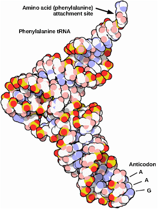
OpenStax · 18.2 Formation of New Species ↗
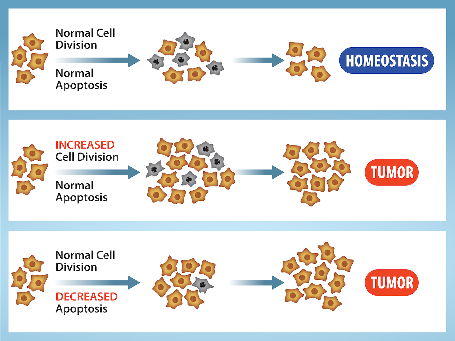
Instructional page including learning objectives, examples, figures, source tables and questions. Site navigation and embedded media players are omitted; source media links remain available.

Learning Objectives

By the end of this section, you will be able to do the following:

  • Define species and describe how scientists identify species as different
  • Describe genetic variables that lead to
  • Identify prezygotic and postzygotic reproductive barriers
  • Explain allopatric and
  • Describe adaptive radiation

Although all life on earth shares various genetic similarities, only certain organisms combine genetic information by sexual reproduction and have offspring that can then successfully reproduce. Scientists call such organisms members of the same biological species.

Species and the Ability to Reproduce

A species is a group of individual organisms that interbreed and produce fertile, viable offspring. According to this definition, one species is distinguished from another when, in nature, it is not possible for matings between individuals from each species to produce fertile offspring.

Members of the same species share both external and internal characteristics, which develop from their . The closer relationship two organisms share, the more they have in common, just like people and their families. People’s is likely to be more like their father or mother’s than their cousin or grandparent’s . Organisms of the same species have the highest level of alignment and therefore share characteristics and behaviors that lead to successful reproduction.

Species’ appearance can be misleading in suggesting an ability or inability to mate. For example, even though domestic dogs (Canis lupus familiaris) display phenotypic differences, such as size, build, and coat, most dogs can interbreed and produce viable puppies that can mature and sexually reproduce (Figure 18.9).

Photo a shows a poodle with curly short fur. Photo b shows a cocker spaniel with long, wavy fur that has light brown parts and cream-colored markings on the face, forepaws, belly, hind legs, and tail. The poodle has longer legs than the cocker spaniel. The cockapoo in photo c has curly hair, like the poodle, and short legs, like the cocker spaniel.
Figure 18.9 — 18.2 Formation of New Species
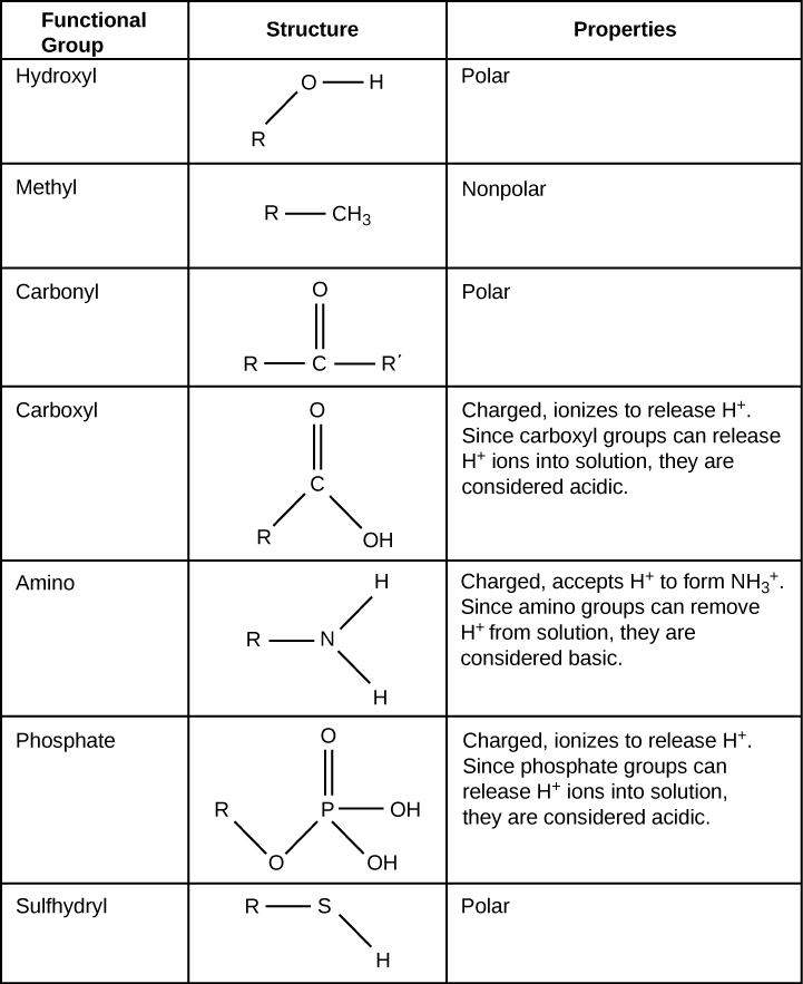
Figure 18.9 The (a) poodle and (b) cocker spaniel can reproduce to produce a breed known as (c) the cockapoo. (credit a: modification of work by Sally Eller, Tom Reese; credit b: modification of work by Jeremy McWilliams; credit c: modification of work by Kathleen Conklin)

Mary Ann Clark, Matthew Douglas, and Jung Choi, Biology 2E, OpenStax. (credit a: modification of work by Sally Eller, Tom Reese; credit b: modification of work by Jeremy McWilliams; credit c: modification of work by Kathleen Conklin) · CC BY-NC-SA 4.0 · Original image ↗ · Access for free ↗

In other cases, individuals may appear similar although they are not members of the same species. For example, even though bald eagles (Haliaeetus leucocephalus) and African fish eagles (Haliaeetus vocifer) are both birds and eagles, each belongs to a separate species group (Figure 18.10). If humans were to artificially intervene and fertilize a bald eagle's egg with an African fish eagle's sperm and a chick did hatch, that offspring, called a hybrid (a cross between two species), would probably be infertile—unable to successfully reproduce after it reached maturity. Different species may have different that are active in development; therefore, it may not be possible to develop a viable offspring with two different sets of directions. Thus, even though may take place, the two species still remain separate.

Photo a shows a picture of the African fish eagle in flight, and photo b shows the bald eagle perched on a post.  Both birds have dark brown feathers on their bodies and wings, and white feathered heads.
Figure 18.10 — 18.2 Formation of New Species
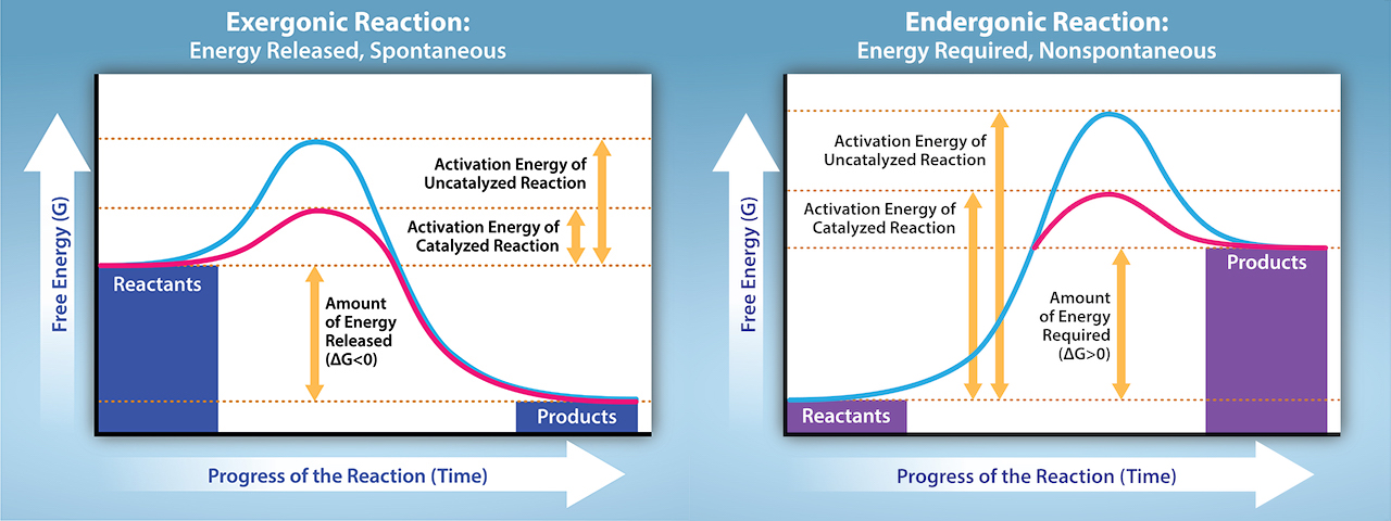
Figure 18.10 The (a) African fish eagle is similar in appearance to the (b) bald eagle, but the two birds are members of different species. (credit a: modification of work by Nigel Wedge; credit b: modification of work by U.S. Fish and Wildlife Service)

Mary Ann Clark, Matthew Douglas, and Jung Choi, Biology 2E, OpenStax. (credit a: modification of work by Nigel Wedge; credit b: modification of work by U.S. Fish and Wildlife Service) · CC BY-NC-SA 4.0 · Original image ↗ · Access for free ↗

Populations of species share a pool: a collection of all the variants in the species. Again, the basis to any changes in a group or population of organisms must be genetic for this is the only way to share and pass on traits. When variations occur within a species, they can only pass to the next generation along two main pathways: asexual reproduction or sexual reproduction. The change will pass on asexually simply if the reproducing cell possesses the changed trait. For the changed trait to pass on by sexual reproduction, a , such as a sperm or egg cell, must possess the changed trait. In other words, sexually-reproducing organisms can experience several genetic changes in their body cells, but if these changes do not occur in a sperm or egg cell, the changed trait will never reach the next generation. Only heritable traits can evolve. Therefore, reproduction plays a paramount role for genetic change to take root in a population or species. In short, organisms must be able to reproduce with each other to pass new traits to offspring.

The biological definition of species, which works for sexually reproducing organisms, is a group of actual or potential interbreeding individuals. There are exceptions to this rule. Many species are similar enough that hybrid offspring are possible and may often occur in nature, but for the majority of species this rule generally holds. The presence in nature of hybrids between similar species suggests that they may have descended from a single interbreeding species, and the process may not yet be completed.

Given the extraordinary diversity of life on the planet there must be mechanisms for : the formation of two species from one original species. Darwin envisioned this process as a branching event and diagrammed the process in the only illustration in On the Origin of Species (Figure 18.11a). Compare this illustration to the diagram of elephant evolution (Figure 18.11b), which shows that as one species changes over time, it branches to form more than one new species, repeatedly, as long as the population survives or until the organism becomes extinct.

Image (a) shows a sketch of lines branching into a tree shape. At the bottom are 11 vertical lines labeled A through L. These then are branched out as they move up across the page through fourteen rows labeled with Roman numerals. Some branches make a straight line from the bottom row to the top row, others keep branching out further at each row, and some are straight partway through the rows until they connect to an existing branch or form no connection and instead stop. The top four rows contain lines branching out from 6 locations on row 11 to 15 individual final designations on row 14. Illustration B shows the evolution of modern African and Asian elephants from a common ancestor, the Palaeomastodon. The Palaeomastodon was similar to modern elephants; however, it was smaller and had a long nose instead of a trunk. Side branches of the elephant evolutionary tree gave rise to mastodons and mammoths. The mammoth is more closely related to modern elephants than the mastodon.
Figure 18.11 — 18.2 Formation of New Species

Figure 18.11 The only illustration in Darwin's On the Origin of Species is (a) a diagram showing speciation events leading to biological diversity. The diagram shows similarities to phylogenetic charts that today illustrate the relationships of species. (b) Modern elephants evolved from the Palaeomastodon , a species that lived in Egypt 35–50 million years ago.

Mary Ann Clark, Matthew Douglas, and Jung Choi, Biology 2E, OpenStax. · CC BY-NC-SA 4.0 · Original image ↗ · Access for free ↗

For to occur, two new populations must form from one original population and they must evolve in such a way that it becomes impossible for individuals from the two new populations to interbreed. Biologists have proposed mechanisms by which this could occur that fall into two broad categories. (allo- = "other"; -patric = "homeland") involves geographic separation of populations from a parent species and subsequent evolution. (sym- = "same"; -patric = "homeland") involves occurring within a parent species remaining in one location.

Biologists think of events as the splitting of one ancestral species into two descendant species. There is no reason why more than two species might not form at one time except that it is less likely and we can conceptualize multiple events as single splits occurring close in time.

A geographically continuous population has a pool that is relatively homogeneous. , the movement of across a species' range, is relatively free because individuals can move and then mate with individuals in their new location. Thus, an 's frequency at one end of a distribution will be similar to the 's frequency at the other end. When populations become geographically discontinuous, it prevents ' free-flow. When that separation lasts for a period of time, the two populations are able to evolve along different trajectories. Thus, their at numerous genetic gradually become increasingly different as new independently arise by in each population. Typically, environmental conditions, such as climate, resources, predators, and competitors for the two populations will differ causing to favor divergent in each group.

Isolation of populations leading to can occur in a variety of ways: a river forming a new branch, erosion creating a new valley, a group of organisms traveling to a new location without the ability to return, or seeds floating over the ocean to an island. The nature of the geographic separation necessary to isolate populations depends entirely on the organism's biology and its potential for dispersal. If two flying insect populations took up residence in separate nearby valleys, chances are, individuals from each population would fly back and forth continuing . However, if a new lake divided two rodent populations continued would be unlikely; therefore, would be more likely.

Biologists group allopatric processes into two categories: dispersal and vicariance. Dispersal is when a few members of a species move to a new geographical area, and vicariance is when a natural situation arises to physically divide organisms.

Scientists have documented numerous cases of taking place. For example, along the west coast of the United States, two separate spotted owl subspecies exist. The northern spotted owl has genetic and phenotypic differences from its close relative: the Mexican spotted owl, which lives in the south (Figure 18.12).

The northern spotted owl lives in the Pacific Northwest, and the Mexican spotted owl lives in Mexico and the southwestern portion of the United States. The two owls are similar in appearance but with slightly different coloration.
Figure 18.12 — 18.2 Formation of New Species
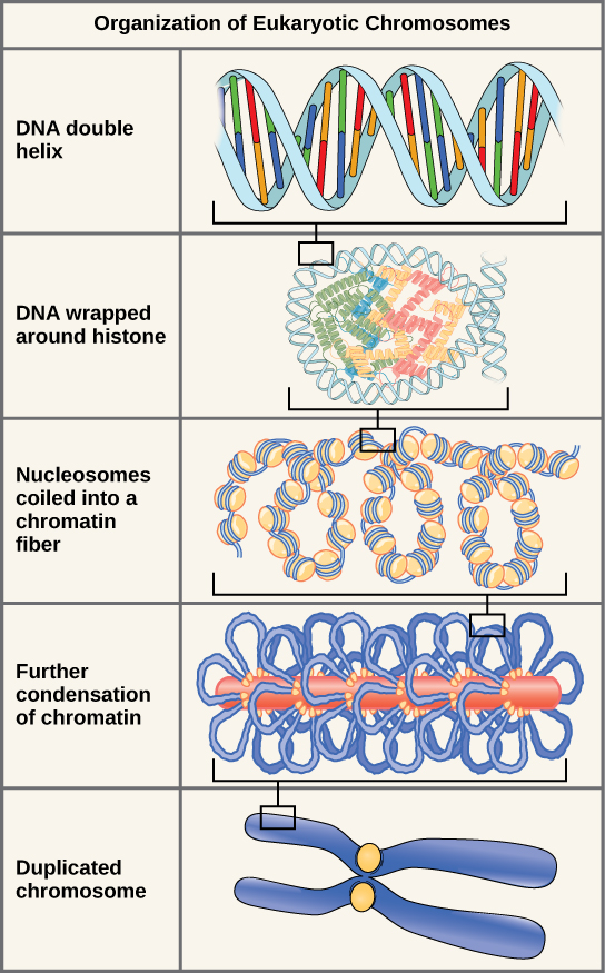
Figure 18.12 The northern spotted owl and the Mexican spotted owl inhabit geographically separate locations with different climates and ecosystems. The owl is an example of allopatric speciation. (credit "northern spotted owl": modification of work by John and Karen Hollingsworth; credit "Mexican spotted owl": modification of work by Bill Radke)

Mary Ann Clark, Matthew Douglas, and Jung Choi, Biology 2E, OpenStax. (credit "northern spotted owl": modification of work by John and Karen Hollingsworth; credit "Mexican spotted owl": modification of work by Bill Radke) · CC BY-NC-SA 4.0 · Original image ↗ · Access for free ↗

Additionally, scientists have found that the further the distance between two groups that once were the same species, the more likely it is that will occur. This seems logical because as the distance increases, the various environmental factors would likely have less in common than locations in close proximity. Consider the two owls: in the north, the climate is cooler than in the south. The types of organisms in each ecosystem differ, as do their behaviors and habits. Also, the hunting habits and prey choices of the southern owls vary from the northern owls. These variances can lead to evolved differences in the owls, and likely will occur.

Adaptive Radiation

In some cases, a population of one species disperses throughout an area, and each finds a distinct niche or isolated habitat. Over time, the varied demands of their new lifestyles lead to multiple events originating from a single species. We call this adaptive radiation because many evolve from a single point of origin; thus, causing the species to radiate into several new ones. Island archipelagos like the Hawaiian Islands provide an ideal context for adaptive radiation events because water surrounds each island which leads to geographical isolation for many organisms. The Hawaiian honeycreeper illustrates one example of adaptive radiation. From a single species, the founder species, numerous species have evolved, including the six in Figure 18.13.

The illustration shows a wheel with the founder species at the hub. The spokes of the wheel are six modern honeycreeper bird species that evolved from the founder bird species. Five of these birds eat insects and or nectar and have long, thick beaks; these are the ‘Apapane, ‘Iwi, ‘Amakihi, ‘Akiapola'au and Maui Parrotbill. The Nihoa Finch has a short, fat beak and eats insects, seeds, and bird eggs.
Figure 18.13 — 18.2 Formation of New Species
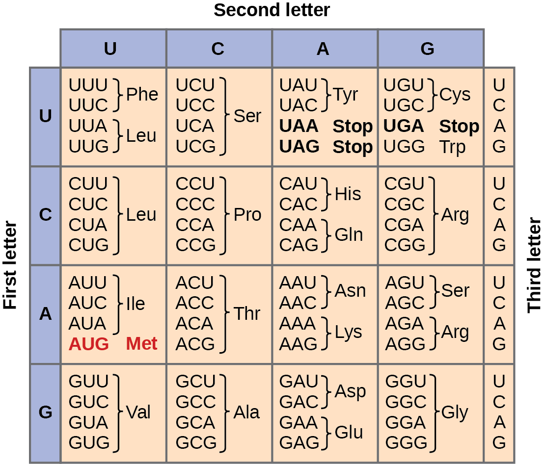
Figure 18.13 The honeycreeper birds illustrate adaptive radiation. From one original species of bird, multiple others evolved, each with its own distinctive characteristics.

Mary Ann Clark, Matthew Douglas, and Jung Choi, Biology 2E, OpenStax. · CC BY-NC-SA 4.0 · Original image ↗ · Access for free ↗

Notice the differences in the species’ beaks in Figure 18.13. Evolution in response to based on specific food sources in each new habitat led to evolution of a different beak suited to the specific food source. The seed-eating bird has a thicker, stronger beak which is suited to break hard nuts. The nectar-eating birds have long beaks to dip into flowers to reach the nectar. The insect-eating birds have beaks like swords, appropriate for stabbing and impaling insects. Darwin’s finches are another example of adaptive radiation in an archipelago.

Link to Learning

Watch this video to see how scientists use evidence to understand how birds evolved.

Can divergence occur if no physical barriers are in place to separate individuals who continue to live and reproduce in the same habitat? The answer is yes. We call the process of within the same space sympatric. The prefix “sym” means same, so “sympatric” means “same homeland” in contrast to “allopatric” meaning “other homeland.” Scientists have proposed and studied many mechanisms.

One form of can begin with a serious error during cell division. In a normal cell division event replicate, pair up, and then separate so that each new cell has the same number of . However, sometimes the pairs separate and the end cell has extra sets of in a condition that we call (Figure 18.14).

Visual Connection

Aneuploidy results when chromosomes fail to separate correctly during meiosis. As a result, one gamete has one too many chromosomes, shown as n plus 1, and the other has one too few, shown as n minus 1. When the n + 1 gamete fuses with a normal gamete, the resulting zygote has 2 n + 1 chromosomes. When the n minus 1 gamete fuses with a normal gamete, the resulting zygote has 2 n minus 1 chromosomes.
Figure 18.14 — 18.2 Formation of New Species
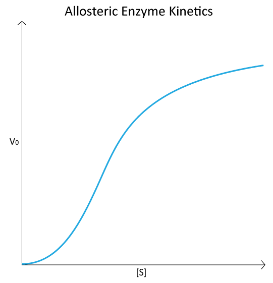
Figure 18.14 Aneuploidy results when the gametes have too many or too few chromosomes due to nondisjunction during meiosis. In this example, the resulting offspring will have 2 n +1 or 2 n -1 chromosomes.

Mary Ann Clark, Matthew Douglas, and Jung Choi, Biology 2E, OpenStax. · CC BY-NC-SA 4.0 · Original image ↗ · Access for free ↗

Which is most likely to survive, offspring with 2n+1 or offspring with 2n-1 ?

is a condition in which a cell or organism has an extra set, or sets, of . Scientists have identified two main types of that can lead to reproductive isolation of an individual in the state. Reproductive isolation is the inability to interbreed. In some cases, a polyploid individual will have two or more complete sets of from its own species in a condition that we call autopolyploidy (Figure 18.15). The prefix “auto-” means “self,” so the term means multiple from one’s own species. results from an error in in which all of the move into one cell instead of separating.

Autopolyploidy results in offspring with two sets of chromosomes. In the example shown, a diploid parent, 2 n produces polyploid offspring 4 n.
Figure 18.15 — 18.2 Formation of New Species
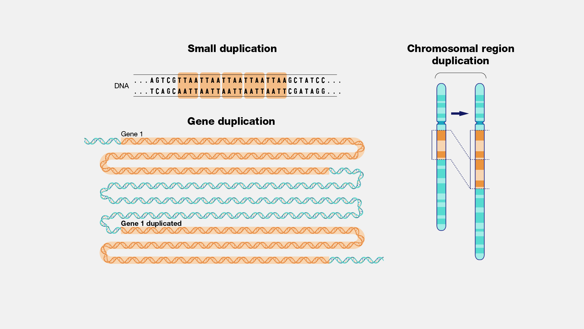
Figure 18.15 Autopolyploidy results when mitosis is not followed by cytokinesis.

Mary Ann Clark, Matthew Douglas, and Jung Choi, Biology 2E, OpenStax. · CC BY-NC-SA 4.0 · Original image ↗ · Access for free ↗

For example, if a plant species with 2n = 6 produces autopolyploid that are also (2n = 6, when they should be n = 3), the now have twice as many as they should have. These new will be incompatible with the normal that this plant species produces. However, they could either self-pollinate or reproduce with other autopolyploid plants with having the same number. In this way, can occur quickly by forming offspring with 4n that we call a tetraploid. These individuals would immediately be able to reproduce only with those of this new kind and not those of the ancestral species.

The other form of occurs when individuals of two different species reproduce to form a viable offspring that we call an allopolyploid. The prefix “allo-” means “other” (recall from allopatric): therefore, an allopolyploid occurs when from two different species combine. Figure 18.16 illustrates one possible way an allopolyploid can form. Notice how it takes two generations, or two reproductive acts, before the viable fertile hybrid results.

Alloploidy results from viable matings between two species with different numbers of chromosomes. In the example shown, species one has two pairs of chromosomes, and species two has three pairs of chromosomes. When an unreduced gamete from species one (with two pairs of chromosomes) fuses with a normal gamete from species two (with three unpaired chromosomes), a hybrid zygote with seven chromosomes results. An offspring from this mating produces an unreduced gamete with seven chromosomes. If this unreduced gamete fuses with a normal gamete from species one, with three chromosomes, the resulting offspring will have ten viable chromosomes (five pairs of chromosomes).
Figure 18.16 — 18.2 Formation of New Species

Figure 18.16 Alloploidy results when two species mate to produce viable offspring. In this example, a normal gamete from one species fuses with a polyploidy gamete from another. Two matings are necessary to produce viable offspring.

Mary Ann Clark, Matthew Douglas, and Jung Choi, Biology 2E, OpenStax. · CC BY-NC-SA 4.0 · Original image ↗ · Access for free ↗

The cultivated forms of wheat, cotton, and tobacco plants are all allopolyploids. Although occurs occasionally in animals, it takes place most commonly in plants. (Animals with any of the types of aberrations that we describe here are unlikely to survive and produce normal offspring.) Scientists have discovered more than half of all plant species studied relate back to a species evolved through . With such a high rate of in plants, some scientists hypothesize that this mechanism takes place more as an than as an error.

Reproductive Isolation

Given enough time, the genetic and phenotypic divergence between populations will affect characters that influence reproduction: if individuals of the two populations were brought together, mating would be less likely, but if mating occurred, offspring would be nonviable or infertile. Many types of diverging characters may affect the reproductive isolation, the ability to interbreed, of the two populations.

Reproductive isolation can take place in a variety of ways. Scientists organize them into two groups: and . Recall that a is a fertilized egg: the first cell of an organism's development that reproduces sexually. Therefore, a is a mechanism that blocks reproduction from taking place. This includes barriers that prevent fertilization when organisms attempt reproduction. A occurs after formation. This includes organisms that don’t survive the embryonic stage and those that are born sterile.

Some types of prevent reproduction entirely. Many organisms only reproduce at certain times of the year, often just annually. Differences in breeding schedules, which we call temporal isolation, can act as a form of reproductive isolation. For example, two frog species inhabit the same area, but one reproduces from January to March; whereas, the other reproduces from March to May (Figure 18.17).

Photo a shows Rana aurora, a beige frog with green spots. Photo b shows Rana boylii, a brown frog.
Figure 18.17 — 18.2 Formation of New Species
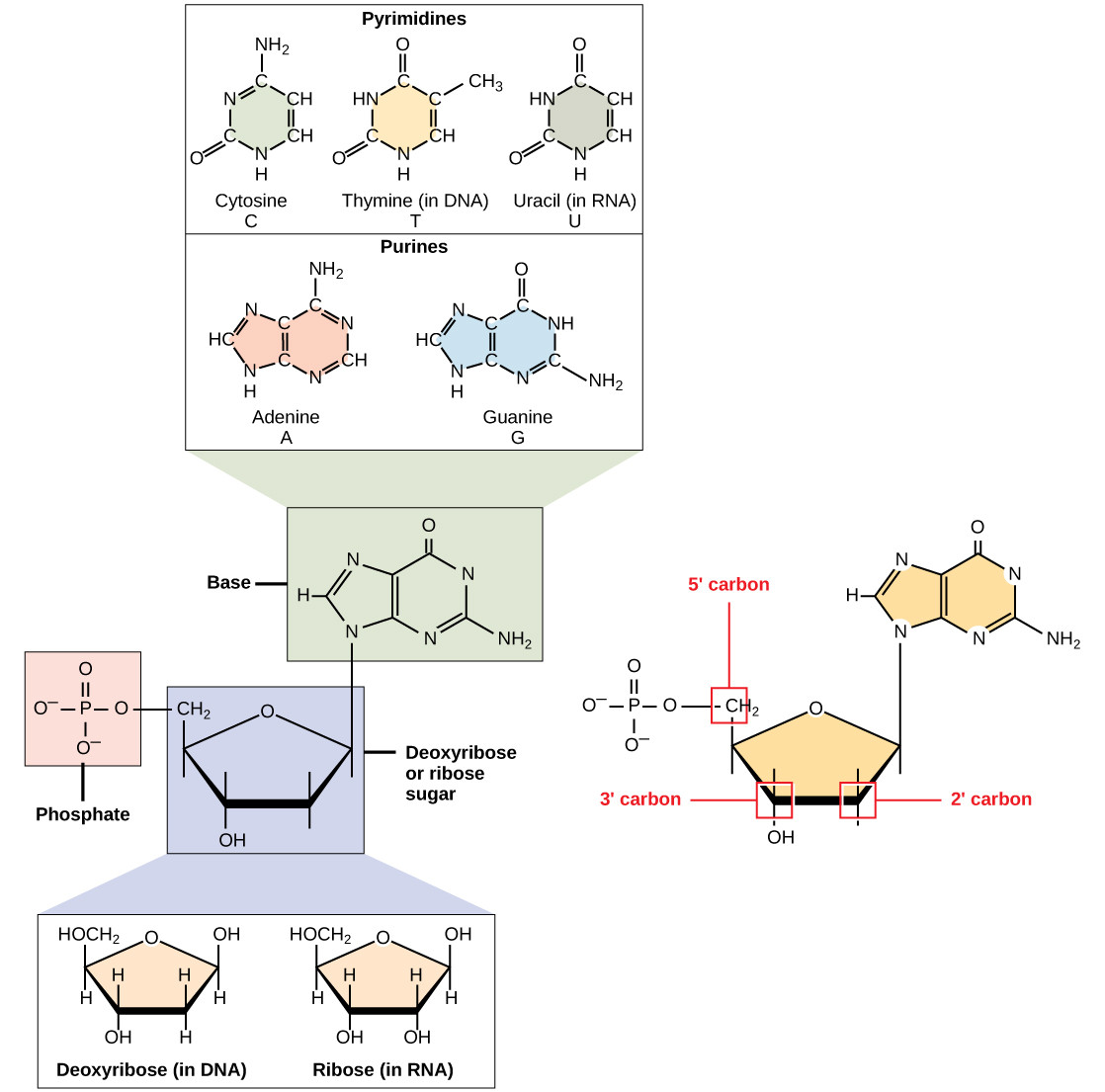
Figure 18.17 These two related frog species exhibit temporal reproductive isolation. (a) Rana aurora breeds earlier in the year than (b) Rana boylii . (credit a: modification of work by Mark R. Jennings, USFWS; credit b: modification of work by Alessandro Catenazzi)

Mary Ann Clark, Matthew Douglas, and Jung Choi, Biology 2E, OpenStax. (credit a: modification of work by Mark R. Jennings, USFWS; credit b: modification of work by Alessandro Catenazzi) · CC BY-NC-SA 4.0 · Original image ↗ · Access for free ↗

In some cases, populations of a species move or are moved to a new habitat and take up residence in a place that no longer overlaps with the same species' other populations. We call this situation habitat isolation. Reproduction with the parent species ceases, and a new group exists that is now reproductively and genetically independent. For example, a cricket population that was divided after a flood could no longer interact with each other. Over time, forces, , and will likely result in the two groups diverging (Figure 18.18).

Illustration A shows the black Gryllus pennsylvanicus cricket on sandy soil, and illustration B shows the beige Gryllus firmus cricket in grass.
Figure 18.18 — 18.2 Formation of New Species
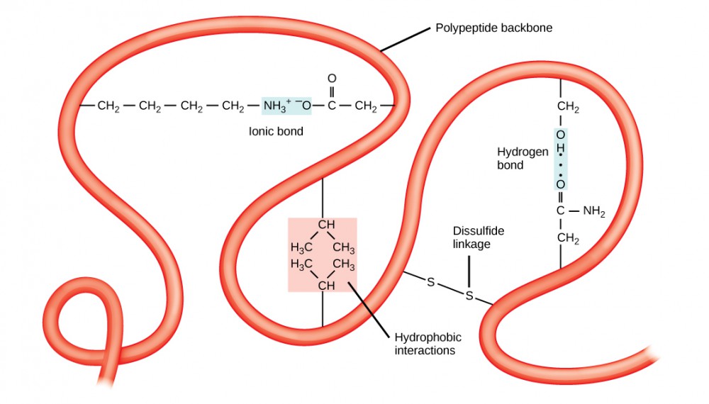
Figure 18.18 Speciation can occur when two populations occupy different habitats. The habitats need not be far apart. The cricket (a) Gryllus pennsylvanicus prefers sandy soil, and the cricket (b) Gryllus firmus prefers loamy soil. The two species can live in close proximity, but because of their different soil preferences, they became genetically isolated.

Mary Ann Clark, Matthew Douglas, and Jung Choi, Biology 2E, OpenStax. · CC BY-NC-SA 4.0 · Original image ↗ · Access for free ↗

Behavioral isolation occurs when the presence or absence of a specific behavior prevents reproduction. For example, male fireflies use specific light patterns to attract females. Various firefly species display their lights differently. If a male of one species tried to attract the female of another, she would not recognize the light pattern and would not mate with the male.

Other work when differences in their cells (eggs and sperm) prevent fertilization from taking place. We call this a gametic barrier. Similarly, in some cases closely related organisms try to mate, but their reproductive structures simply do not fit together. For example, damselfly males of different species have differently shaped reproductive organs. If one species tries to mate with the female of another, their body parts simply do not fit together. (Figure 18.19).

Illustrations show four different types of damselfly reproductive organs. Each organ has a hook, but the shape and length of the hook varies, as does the shape of the organ itself.
Figure 18.19 — 18.2 Formation of New Species
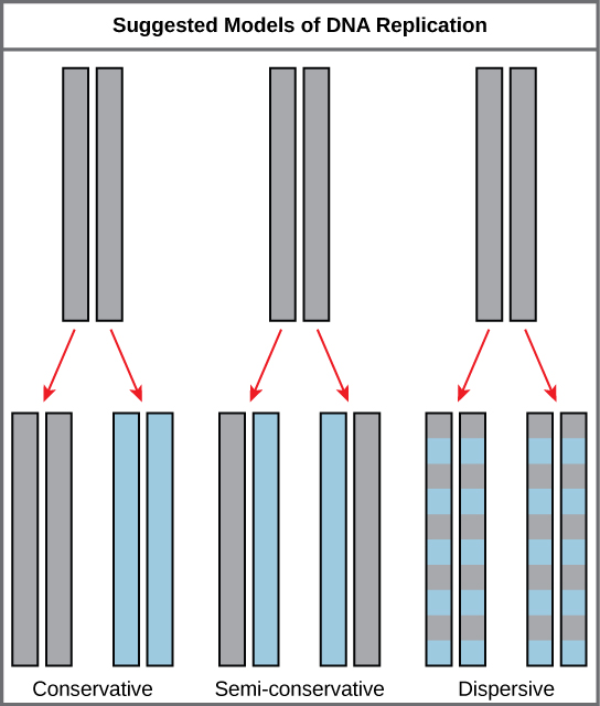
Figure 18.19 The shape of the male reproductive organ varies among male damselfly species, and is only compatible with the female of that species. Reproductive organ incompatibility keeps the species reproductively isolated.

Mary Ann Clark, Matthew Douglas, and Jung Choi, Biology 2E, OpenStax. · CC BY-NC-SA 4.0 · Original image ↗ · Access for free ↗

In plants, certain structures aimed to attract one type of pollinator simultaneously prevent a different pollinator from accessing the pollen. The tunnel through which an animal must access nectar can vary widely in length and diameter, which prevents the plant from cross-pollinating with a different species (Figure 18.20).

Illustration a shows a bee collecting pollen from a bright purple foxglove flower. The bee's body fits inside the bell like flower. Illustration B shows a hummingbird drinking nectar from a long tube like trumpet creeper flower.
Figure 18.20 — 18.2 Formation of New Species
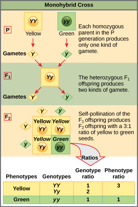
Figure 18.20 Some flowers have evolved to attract certain pollinators. The (a) wide foxglove flower is adapted for pollination by bees, while the (b) long, tube-shaped trumpet creeper flower is adapted for pollination by hummingbirds.

Mary Ann Clark, Matthew Douglas, and Jung Choi, Biology 2E, OpenStax. · CC BY-NC-SA 4.0 · Original image ↗ · Access for free ↗

When fertilization takes place and a forms, can prevent reproduction. Hybrid individuals in many cases cannot form normally in the womb and simply do not survive past the embryonic stages. We call this hybrid inviability because the hybrid organisms simply are not viable. In another postzygotic situation, reproduction leads to hybrid birth and growth that is sterile. Therefore, the organisms are unable to reproduce offspring of their own. We call this hybrid sterility.

Habitat Influence on

may also take place in ways other than . For example, consider a fish species that lives in a lake. As the population grows, competition for food increases. Under pressure to find food, suppose that a group of these fish had the genetic flexibility to discover and feed off another resource that other fish did not use. What if this new food source was located at a different depth of the lake? Over time, those feeding on the second food source would interact more with each other than the other fish; therefore, they would breed together as well. Offspring of these fish would likely behave as their parents: feeding and living in the same area and keeping separate from the original population. If this group of fish continued to remain separate from the first population, eventually might occur as more genetic differences accumulated between them.

This scenario does play out in nature, as do others that lead to reproductive isolation. One such place is Lake Victoria in Africa, famous for its of cichlid fish. Researchers have found hundreds of events in these fish, which have not only happened in great number, but also over a short period of time. Figure 18.21 shows this type of among a cichlid fish population in Nicaragua. In this locale, two types of cichlids live in the same geographic location but have come to have different morphologies that allow them to eat various food sources.

Illustrations show two species of cichlid fish which are similar in appearance except that one has thin lips, and one has thick lips.
Figure 18.21 — 18.2 Formation of New Species
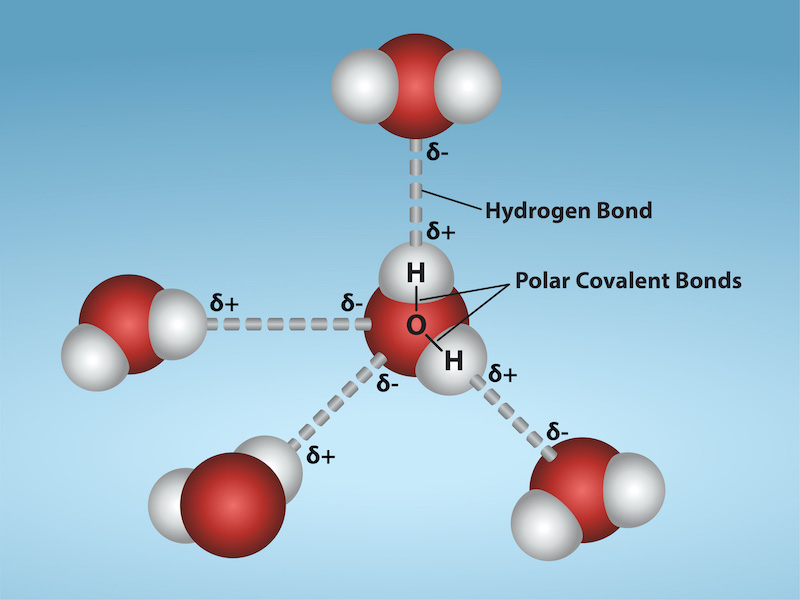
Figure 18.21 Cichlid fish from Lake Apoyeque, Nicaragua, show evidence of sympatric speciation. Lake Apoyeque, a crater lake, is 1800 years old, but genetic evidence indicates that a single population of cichlid fish populated the lake only 100 years ago. Nevertheless, two populations with distinct morphologies and diets now exist in the lake, and scientists believe these populations may be in an early stage of speciation.
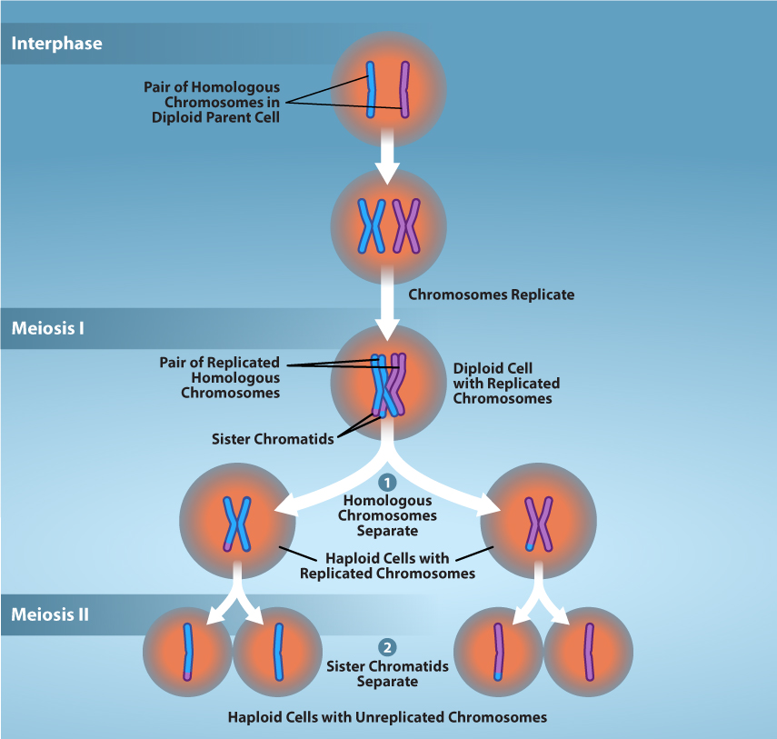
Mary Ann Clark, Matthew Douglas, and Jung Choi, Biology 2E, OpenStax. · CC BY-NC-SA 4.0 · Original image ↗ · Access for free ↗